Introduction

About the Instructor

Where this lecture is going

The Task-Based Framework

A job is a bundle of tasks. AI substitutes some tasks, complements others — and which tasks determines everything.

Implications for Finance Professionals

Tools that compress low-value tasks free capacity for high-value ones where human judgment dominates.

Tetlock (2007): the news has a mood, and the mood has a price

A simple experiment: measure how negative the Wall Street Journal's daily market column sounds, then ask whether tomorrow's market moves with it.

Early Approaches: Keyword Counting and Dictionary Methods

The Shift to Statistical and Neural Methods

By the mid-2000s NLP moved beyond dictionaries to methods that learn structure from the data — no hand-coding required.

• Boudoukh et al. (2013): LDA on firm-level news identified which stories actually move stock prices
• Hansen, McMahon & Prat (2018): LDA on FOMC transcripts revealed deliberation structure — who is hawkish, who is dovish — invisible to word-counting

The Quantitative Growth of Financial Text

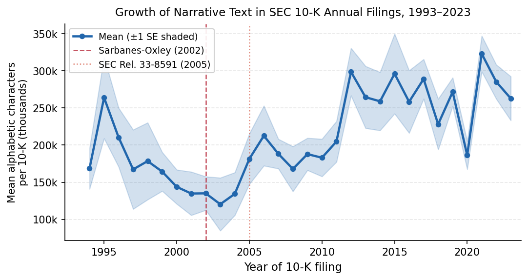
More text means more signal — but also more work for any human reader. That gap is where NLP tools earn their keep.

The Information Content of Earnings Calls, News, and Filings

If markets are efficient, why does news tone predict returns?

Efficient-markets theory (Fama, 1970) says prices already reflect public information. Yet the data keeps finding that text predicts returns. Three reconciling reasons:

1. Processing costs & limited attention. A 200-page 10-K is expensive to read. Not everyone does — so signals persist until the technology to read at scale spreads. Li, Lundholm & Minnis (2013): textual signals are strongest precisely for documents that are longest and most complex.
2. Soft information & disagreement. Is a cautious tone genuine worry, or expectation management? When readers disagree, price reflects the average belief, not the sharpest one.
3. Latent information. Regulation limits explicit selective disclosure (Reg FD), so meaning leaks through word choice, omissions, and rhetorical structure.

Text as a Signal: Evidence from the Literature

1. Negative tone → negative short-run returns, then reversal. Tetlock (2007).
2. Finance dictionaries beat general ones. Loughran–McDonald (2011).
3. Call tone predicts future earnings surprises and deception. Larcker & Zakolyukina (2012): deceptive speech has distinct linguistic markers.
4. LLM-based signals add fresh predictive power. Lopez-Lira & Tang (2023): ChatGPT headline sentiment predicts next-day returns. Absent in GPT-1 and BERT — an emergent property of scale.

A "textual signal," defined once and used all course

Strip away the jargon: a text signal is just a recipe that turns a document into numbers.

Four ways a "signal" can fool you

Cleaning text before you can count it

Every method starts by standardising raw text into a tidy vocabulary.

1. Case folding — "Revenue" = "revenue"
2. Stop-word removal — drop "the", "and", "of"… (100–300 words)
3. Stemming / lemmatisation — earnings, earned, earns → earn
4. Vocabulary truncation — keep the common types, discard the rare ones

Vocabulary, Tokens, and the Bag-of-Words Model

Tip every document into a bag, count each word, forget the order. Crude — but a strong baseline.

One-Hot Encoding

Bag-of-words counted words — but what is a single word, to a computer? It can't read "revenue"; it reads numbers. Fix a vocabulary of \(V\) words, then represent word number \(k\) as a vector that is all zeros except a single 1 in slot \(k\).

To a computer, "revenue" and "income" are total strangers

Under one-hot encoding every word is its own dimension, so no two distinct words share any similarity — "revenue" is as far from "income" as it is from "penguin."

TF-IDF Weighting

Raw counts are dominated by common words. TF-IDF up-weights words that are frequent in this document but rare across the corpus — the ones that actually distinguish it.

• A word in every document → IDF = 0 (says nothing distinctive)
• A word in one document → maximal weight (highly distinctive)
• Cosine similarity on TF-IDF vectors is length-invariant — the vector space model (Salton et al., 1975)

The shared blind spots of every classical method

Distributional Semantics and the Embedding Idea

An embedding maps each word to a point in a few-hundred-dimensional space where direction and distance encode meaning.

Word2Vec and GloVe

Train a model to guess the words surrounding a target word. To do that well it's forced to place related words near each other. That arrangement is the embedding.

Factorising co-occurrence counts instead of streaming windows

Word2Vec processes one window at a time; GloVe counts all co-occurrences across the entire corpus first, then fits the geometry in one pass.

• Key insight: the ratio of co-occurrence probabilities \(P_{ik}/P_{jk}\) encodes relational meaning more faithfully than raw probabilities
• Minimise a weighted squared loss between the dot product of word vectors and \(\log X_{ij}\)
• Pennington, Socher & Manning (2014): recommended \(\alpha = 0.75\), \(x_{\max} = 100\)

"Risk" means something different on Wall Street

Three ways to adapt

• Train from scratch on a financial corpus (e.g. BloombergGPT, FinancialPhraseBank embeddings)
• Fine-tune a general model (FinBERT: BERT re-trained on news, 10-Ks, calls)
• Retrofit — nudge synonyms together / antonyms apart using a financial lexicon

Applications

• Ke et al. (2019): supervised text-mining learns which words in financial news best predict asset returns — outperforms bag-of-words baselines out-of-sample
• Manela & Moreira (2017): embedding-based text features construct a news-implied measure of disaster risk (news-implied volatility)

Case Study: Visualising a Word Analogy with PCA

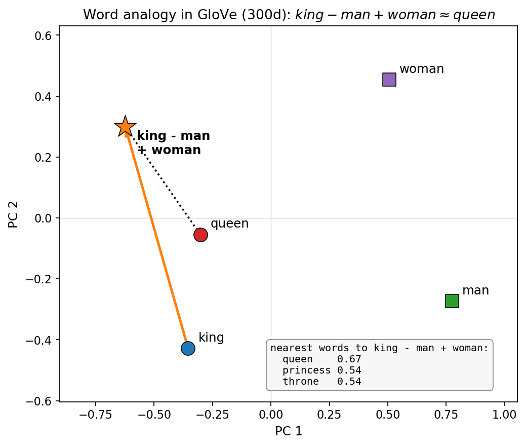
Load pre-trained GloVe (300d), compute the analogy in full vector space, then project to 2D with PCA — the arithmetic lands next to queen (cosine similarity 0.67).

The Recurrence and Why Gradients Vanish

Each token folds into a running hidden state — a summary of everything read so far. But carrying that summary across 500 tokens breaks.

The LSTM Fix, in One Idea

Instead of repeatedly multiplying the hidden state, the LSTM cell state is updated additively — gradients flow like water through an open pipe.

• Hochreiter & Schmidhuber (1997): Long Short-Term Memory adds a cell state \(\mathbf{c}_t\) updated via learned gates
• Forget gate: what fraction of the old cell to erase
• Input gate: what new information to write into the cell
• Output gate: what the cell exposes as the hidden state \(\mathbf{h}_t\)
• When the forget gate stays open, the cell state behaves like a near-lossless gradient highway

Attention as Content-Based Lookup

Each token asks a question (query), every token posts an answer (key + value); the update is a weighted average of all values, weighted by how well the query matches each key.

Bahdanau, Cho & Bengio (2015): the original attention mechanism for sequence-to-sequence MT. Vaswani et al. (2017): generalised to the Transformer, which discards recurrence entirely.

Multiple Heads, Multiple Relations

A single attention head can track only one kind of relationship. Multi-head attention runs several in parallel on lower-dimensional projections.

• In financial text: one head may follow temporal links (prior quarter vs. current quarter), another entity coreference (the company, it, JPMorgan), another negation scope (did not, failed to)
• BERT (Devlin et al., 2019): 12-layer Transformer encoder pre-trained with Masked LM (15% of tokens masked); bidirectionality makes it exceptional for classification
• FinBERT (Yang et al., 2020): BERT further pre-trained on Reuters news, 10-K filings, and earnings calls — achieves state-of-the-art sentiment on Financial PhraseBank

How a model is trained determines what it's good at

LLaMA, BloombergGPT, FinGPT — and why data sovereignty matters

Routing proprietary trading data through a third-party API is a compliance problem. Open-weight models run on your servers.

A sentiment query in ten lines of Python

All three APIs share the same structure: a list of role-tagged messages in, a structured response out.

import openai
client = openai.OpenAI()
resp = client.chat.completions.create(
    model="gpt-5.6-luna",  # fast, low-cost tier
    messages=[
      {"role": "system",
       "content": "You are a financial analyst."},
      {"role": "user",
       "content": "Sentiment of 'Revenue fell 12%.'?"
                  " One word."},
    ])
# -> 'Negative'

from transformers import pipeline
# HuggingFace — runs locally
clf = pipeline("text-classification",
               model="ProsusAI/finbert")
print(clf("Revenue fell 12%."))
# -> [{'label': 'negative',
#      'score': 0.95}]

Token Costs and Latency Trade-offs

Illustrative mid-2026 list prices; model names and rates change fast — verify current values before production deployment.

Hallucination: Taxonomy and Detection

An LLM hallucination is an output that is fluent and coherent but factually incorrect, unverifiable, or unsupported by the input context.

Context Window Limitations

Most standard filings fit in modern context windows — but very long documents still require chunking, and placement of relevant facts matters.

The Regulatory Landscape

Deploying an LLM in a client-facing or regulatory context is not just a technical decision — it carries legal obligations.

What we covered — and where Lecture 2 goes

From dictionaries to neural methods — a timeline

Each generation fixes the core limitation of the one before it.

TF-IDF on three tiny sentences

Full computation in Practical Session 1.

Reading PCA plots of embedding space with care

Project 30 financial terms to 2D via PCA on GloVe vectors and colour by theme — consistent clusters appear, but axes need careful interpretation.

• option, futures, derivative → tight cluster
• default, credit → together, away from equities
• merger, acquisition → nearly identical vectors
• Rates (yield, spread, inflation, interest rate) → the most cohesive group

Full code: code/practicals/01-intro/practical.ipynb