Training and Fine-Tuning Large Language Models
What we'll do in the next hour
Four skills, end to end: read a scaling law as a budget, size a LoRA adapter, run a real fine-tune on a finance task, and reason about preference data for alignment.
Recap — the formulas you'll lean on
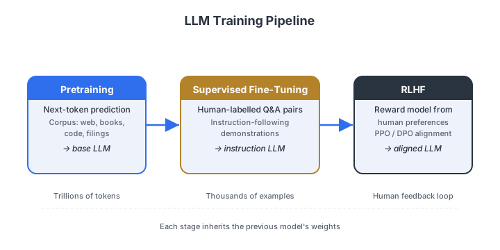
Three stages from raw text to aligned model
Every modern finance LLM passes through three distinct phases — understanding which phase you are in determines which tools and metrics matter.
LoRA: train a tiny patch, not the whole model
Instead of editing billions of frozen weights, LoRA bolts on two small matrices and only trains those — a cheap, removable "patch."
- The base weights stay frozen; only the patch learns
- Start the patch at zero, so day-one behaviour is unchanged
- At inference you can merge the patch in — zero extra cost
- Rank \(r\) is the dial: typical 4, 8, 16, 32
Chinchilla: model size and data should grow together
For a fixed compute budget there's a sweet spot — roughly 20 tokens of training data per model parameter. Too big a model on too little data wastes the budget.
| Objective | Architecture | Finance use |
|---|---|---|
| CLM (causal) | Decoder-only | Generation, chat, BloombergGPT |
| MLM (masked) | Encoder-only | Classification, NER, FinBERT |
| Span corruption | Encoder-decoder | QA, summarisation |
Problems — do the arithmetic yourself
How many parameters does a LoRA patch actually train?
Model: LLaMA-7B, 32 transformer layers, hidden dimension \(d = 4096\). Each layer has four square projection matrices.
- Query \(W_Q\), Key \(W_K\)
- Value \(W_V\), Output \(W_O\)
Task: apply LoRA with rank \(r = 4\) to the Q and V projections only.
| Matrix | \(d\) | \(k\) | \(r\) |
|---|---|---|---|
| \(W_Q\) | ? | ? | ? |
| \(W_V\) | ? | ? | ? |
Four questions on the LoRA patch
Using the setup (\(r=4\), Q and V only, 32 layers, \(d=k=4096\)) — work individually or in pairs.
- A. Compute the total trainable LoRA parameters. Show the step-by-step arithmetic.
- B. Express this as a fraction of the 7B total. Is it above or below 0.1%?
- C. Double the rank to \(r = 8\). By what factor does the count change — linear, quadratic, or something else? Justify.
- D. A colleague prefers older adapter modules. Give one concrete reason LoRA wins for inference-time deployment on a high-throughput trading floor where latency is measured in milliseconds.
Given a compute budget, how big should the model be?
Scenario: an investment bank's AI team has a compute budget of \(C = 10^{22}\) FLOPs to train a financial language model.
- Compute \(N^*\) and \(D^*\).
- The team has a 50B-token financial corpus. Are they data-constrained or compute-constrained? (Compare \(D^*\) to 50B.)
- What should they do given that diagnosis?
Pushing the budget further
- B. The team instead trains a 1B-parameter model. By the Chinchilla rule, how many tokens for a compute-optimal run? What is the implied FLOP cost?
- C. A senior researcher argues "train the biggest model possible to maximise accuracy." When is this valid? When is it wrong?
Case study — fine-tune FinBERT with LoRA
Teach a finance model with a tiny removable patch
Load pre-trained FinBERT and apply LoRA fine-tuning on a handful of labelled financial sentences using HuggingFace PEFT.
transformers— loadProsusAI/finbertpeft—LoraConfig, thenget_peft_modeltorch— a hand-written training loop (no Trainer, for transparency)
Three steps, then three diagnostic questions
- Run the code on the next frames
- Observe how many parameters are trainable vs. frozen
- Answer the diagnostic questions that follow
pip install transformers peft torch — no API key required for this case study.
Five labelled sentences (positive / negative / neutral)
import torch
from transformers import AutoTokenizer, AutoModelForSequenceClassification
from peft import LoraConfig, get_peft_model, TaskType

MODEL = "ProsusAI/finbert"
SENTENCES = [
    ("Revenue increased 15% year-over-year.", 0),         # positive
    ("The firm reported a net loss of 200M USD.", 1),     # negative
    ("Operating margins remained broadly stable.", 2),    # neutral
    ("Strong demand drove record quarterly earnings.", 0),# positive
    ("Guidance was withdrawn amid macro uncertainty.", 1),# negative
]
Attach the adapter to query and value only
tokenizer = AutoTokenizer.from_pretrained(MODEL)
model = AutoModelForSequenceClassification.from_pretrained(MODEL, num_labels=3)

lora_cfg = LoraConfig(
    task_type=TaskType.SEQ_CLS,
    r=8,
    lora_alpha=16,
    target_modules=["query", "value"],
    lora_dropout=0.05,
    bias="none",
)
model = get_peft_model(model, lora_cfg)
model.print_trainable_parameters()  # observe trainable % here
print_trainable_parameters() is the whole lesson: a sub-1% slice of the model is learning.
Three epochs, then read the predictions
texts, labels = zip(*SENTENCES)
enc = tokenizer(list(texts), padding=True, truncation=True, return_tensors="pt")
label_tensor = torch.tensor(labels)

optimizer = torch.optim.AdamW(model.parameters(), lr=2e-4)
model.train()
for epoch in range(3):
    out = model(**enc, labels=label_tensor)
    out.loss.backward(); optimizer.step(); optimizer.zero_grad()
    print(f"Epoch {epoch+1}: loss={out.loss.item():.4f}")

model.eval()
with torch.no_grad():
    logits = model(**enc).logits
    preds = logits.argmax(-1)
    id2label = {0: "positive", 1: "negative", 2: "neutral"}
    for sent, pred in zip(texts, preds):
        print(f"[{id2label[pred.item()]}] {sent}")
Does the math match what the code reports?
- Q1 — trainable fraction. Compare the reported trainable count to total FinBERT size (\(\approx 110\)M). How does it line up with the theoretical value for LoRA \(r=8\) on query and value across all 12 BERT layers?
- Q2 — rank sweep. Change
r=8tor=4thenr=16; rerun the loop each time. Do predictions change? Does loss fall faster at higher rank? What does that say about rank vs. expressiveness on a tiny dataset?
Is patching all four projections worth the extra cost?
Q3. Change target_modules to all four projections: ["query", "key", "value", "dense"]. How does the trainable count change? Do the predictions improve? Is the extra compute justified?
takala/financial_phrasebank). Evaluate accuracy on a held-out 20% split at \(r = 4, 8, 16\), and plot accuracy vs. trainable parameter count.
Discussion — which adaptation strategy, and why?
Pick the right tool for each desk
For each scenario, choose: zero-shot / few-shot ICL / LoRA fine-tune / full fine-tune — and say why.
- Hedge fund. Classify 10-K risk-factor sections "material" vs. "immaterial" for one covenant type. 50 labelled examples, 2-hour deadline, using GPT-5.6 Luna via API.
- Tier-1 bank. On-premise earnings-call sentiment (no external API), 200,000 docs/month, GDPR data-residency, 20,000 labelled examples.
- Fintech startup. General-purpose financial chatbot; no task-specific labelled data, but access to a pre-trained instruction-tuned LLM.
- Quant research. Test whether a 70B model can replicate an expert's reasoning on novel bond-structuring questions. No labelled data exists.
Solutions — the worked answers
A 7B model fine-tuned by moving ~2 million parameters
| Matrix | \(d\) | \(k\) | \(r\) |
|---|---|---|---|
| \(W_Q\) | 4096 | 4096 | 4 |
| \(W_V\) | 4096 | 4096 | 4 |
The budget says: build small, train fully
Appendix — stretch problems (optional)
Instruction tuning: why format diversity matters
PIXIU / FinMA (Xie et al., 2023) trained on 136,000 financial instruction samples. InvestLM used far fewer but carefully curated samples. Both achieved strong results — for very different reasons.
- A. The Superficial Alignment Hypothesis says instruction quality matters more than quantity. Design a test: what would you measure on a held-out set to distinguish a quality effect from a quantity effect?
- B. A financial chatbot needs to handle three phrasings of the same task: "What is the sentiment?", "Classify as positive/negative/neutral:", "Rate the tone of:". How would you structure an instruction-tuning dataset to handle all three without labelling 3× as much data?
- C. The information-overload effect (Balogh & Didisheim, 2025) shows an inverted-U: accuracy peaks then falls as context length grows. How would you operationalise this finding when designing a RAG pipeline for earnings-call QA?
DPO: aligning a model from preference pairs
You have the LoRA-fine-tuned FinBERT sentiment model from the case study. Now align a small generative finance model with Direct Preference Optimisation on preference pairs \((x, y_w, y_l)\).
- A. In one sentence: what does raising \(\beta\) do to how far \(\pi_\theta\) may drift from \(\pi_{\mathrm{ref}}\)?
- B. Why does DPO need a frozen reference policy \(\pi_{\mathrm{ref}}\) at all? What failure occurs if you drop it?
- C. Construct three plausible \((y_w \succ y_l)\) preference pairs for a financial-advice prompt where "plausible vs. accurate" is the distinguishing axis. Annotate each with the relevant regulatory concern (MiFID II suitability, SR 11-7, or hallucination).