LLMs for Business Valuation
Where this lecture is going
- Valuation frameworks — DCF, multiples, net assets — and where an LLM actually helps.
- Getting the data — pulling clean numbers out of filings and other disclosure sources.
- Cash flows — computing and normalising free cash flow.
- Forecasting — CoT prompting, few-shot vs. fine-tuning, evaluation.
- Tools & arithmetic — why the model must never do the maths itself.
- Scenarios, comparables, pipeline, and cost.
Business valuation: frameworks and the LLM opportunity
What is a business valuation?
Valuation turns financial facts — cash flows, growth, a discount rate — into a single number: what a rational, fully informed buyer would pay for the claim.
- M&A — the spread between buyer and seller defines the zone of possible agreement
- IPOs — banks produce valuation ranges to price new shares
- Portfolio management — model value vs. market price generates trade signals
- Financial reporting — IFRS 13 / ASC 820 Level 3 assets require documented valuation models subject to auditor scrutiny (IASB, 2011)
- Litigation, tax, and regulatory capital — transfer pricing, estate tax, fair-value assessments
You are pricing the future, not the past
A balance sheet records what a company spent. The market prices what it will earn. The whole game is turning today's information into a credible forward estimate.
Every assumption is defensible; every assumption is contestable. Business valuation is the discipline of making assumptions explicit, consistent, and auditable.
Three ways to value a company — and you want all three
The discount rate is itself a model output
WACC is not a market observable — it is derived from the firm's capital structure and the CAPM estimate of equity cost. The cost of equity is the single most consequential input.
- β must be estimated from market data — an LLM should retrieve it, not recall it from training
- ERP and r_f change over time — stale model knowledge is dangerous here
- All computations must go through a code interpreter, never in-context maths
What does an LLM change at each step?
| Step | Traditional approach | LLM contribution |
|---|---|---|
| Data collection | Manual filing parsing | Automated extraction pipeline |
| FCF computation | Spreadsheet formulas | Code interpreter (error-free) |
| FCF normalisation | Analyst reads MD&A | Non-recurring item identification |
| Forecasting | Analyst judgment | CoT prompting + evaluation |
| Scenario analysis | Manual scenarios | Narrative coherence checking |
| Comparable selection | SIC codes + manual | Embedding + LLM hybrid |
| Report generation | Analyst writing | LLM first-draft synthesis |
Extracting financial data from filings
Everything starts with the filings
Structured disclosures are the source of truth. U.S. public companies file through SEC EDGAR — the running example below — but the same pattern applies to other regulators (UK Companies House, EU/ESEF filers, Canada's SEDAR+), company IR pages, earnings-call transcripts, and third-party data vendors. Learn one source well and the extraction pipeline ports to the rest.
- 10-K — annual audited financials + MD&A. Primary source.
- 10-Q — quarterly unaudited interim statements (three per year).
- 8-K — material events within 4 business days (earnings, M&A, CEO changes).
- DEF 14A — proxy: executive comp, board composition, related-party transactions.
- Submissions API:
data.sec.gov/submissions/CIK{cik}.json - Full-text search:
efts.sec.gov/LATEST/search-index?q=... - XBRL companyfacts:
data.sec.gov/api/xbrl/companyfacts/CIK{cik}.json
Getting the pipeline right: rate limits and accession numbers
Every source has quirks that trip up careless implementations. EDGAR's are representative — each of these has an analogue on other portals and vendor APIs.
- User-Agent header required — requests that omit it are throttled or blocked.
- Rate limit — approximately 10 requests per second; exponential backoff for large-scale jobs.
- Accession numbers — format
XXXXXXXXXX-YY-ZZZZZZ; strip hyphens to get the directory path in/Archives/. - Look-ahead bias — always record the filing date, not the fiscal year-end date. Using fiscal year-end in a backtest includes information not yet available to investors.
Why parsing financial tables needs an LLM
Merged cells, multi-level headers, footnotes buried inside cells, non-standard layouts — classical parsers break on the long tail. An LLM reads the table the way a person would.
- Request JSON directly — enables automatic validation against a schema
- Add "Respond only with valid JSON. No markdown code fences." if the model lacks JSON mode
- XBRL as ground truth; LLM extraction fills the gap and acts as cross-check
Assembling a clean, consistent financial data model
Extracting figures from one filing is step one. Assembling them into a schema that can be safely fed into computation — without silent errors — is step two.
- Company identifier — ticker plus a source identifier (e.g., EDGAR CIK, LEI, or vendor ID)
- Fiscal period end date — not all fiscal years end December 31
- Filing date — to prevent look-ahead bias in backtests
- Standardised quantities — units (thousands vs. millions) and sources clearly annotated
- Provenance — XBRL tag or LLM extraction (model + date) for every figure
- Restatement flag — a restated/refiled report (e.g., a 10-K/A) supersedes the original and may change prior figures
Computing free cash flows
Free cash flow to the firm, or to equity?
Free cash flow is the cash a business throws off after paying to keep running and grow. One version belongs to everyone who funded the firm; the other only to shareholders.
FCFF, worked end to end
A hypothetical software company (USD millions) shows how the pieces combine.
| Item | Value (USD M) |
|---|---|
| Revenue | 4,200 |
| EBIT | 840 |
| D&A | 310 |
| CapEx | 180 |
| NWC (current) | 620 |
| NWC (prior) | 540 |
| Tax rate \(\tau\) | 21% |
Enterprise value ≈ $15.2B ≈ 3.6× trailing revenue, consistent with high-quality software-sector medians for firms with strong near-term growth.
"Normalising" EBIT: stripping out the noise
Reported EBIT is full of one-off events that won't repeat. Forecasting off the raw number bakes in distortions. The LLM reads the MD&A and flags what to adjust.
- One-time items — restructuring charges, litigation settlements, impairments. Remove from base EBIT.
- Capitalised operating leases (IFRS 16, ASC 842) — mismatch between reported EBIT, depreciation, and cash flows; must be reconciled carefully.
- Acquired intangible amortisation — from purchase-accounting step-up; often excluded in "cash EBIT" (Koller et al., 2020).
Forecasting cash flows with LLMs
What classical forecasting can and can't do
Simple statistical models project cash flow from its own past. They're honest baselines — but blind to anything not already in the numbers.
Chain-of-thought: force the model to show its work
Wei et al. (2022): prompting the model to reason step by step before answering. For forecasting, this makes it spell out the causal story — so the output is auditable.
- Macro context — how do rates, GDP, and inflation affect revenue and margins?
- Industry dynamics — drivers, headwinds, competition, regulation.
- Firm-specific — competitive position; margin trajectory; CapEx plans from MD&A.
- Synthesis — point estimate + upside (P90) + downside (P10) per year; 2-sentence justification.
Few-shot in-context vs. fine-tuning: when to use which
You can teach an LLM the forecasting task without retraining (few-shot) or with supervised adaptation of its weights (fine-tuning). Each strategy has a different cost–benefit profile.
- 3–10 historical (company, context, forecast) examples prepended to the prompt
- Zero training cost; easy to update; deployment flexibility
- Include diverse macro environments and industry types to reduce forecast variance
- Risk: poorly chosen examples anchor the model to the wrong regime
- Train on labelled (filing, subsequent cash-flow realisation) pairs — captures domain-specific patterns (e.g., MD&A language and earnings surprises)
- LLM signals carry return-predictive information even without fine-tuning (López-Lira and Tang, 2023)
- LoRA / PEFT (Hu et al., 2022): train only a small fraction of parameters — competitive performance at a fraction of the compute cost
How to grade a forecast
Three metrics, each answering a different question: how far off, how far off in dollars, and did we at least get the direction right.
| Metric | Problem | When most useful |
|---|---|---|
| MAPE | Undefined when \(y_t \approx 0\) | Stable, positive cash flows |
| RMSE | Scale-dependent | Within-company comparison |
| DA | Scale-invariant | Investment-decision relevance |
Tool-augmented agents for financial arithmetic
Why you can't trust an LLM with arithmetic
An LLM predicts the next word. Arithmetic is a deterministic algorithm. It can pattern-match simple sums, but reliability collapses as the computation grows.
- A 5-year DCF involves approximately 15–20 chained arithmetic operations
- An incorrectly applied tax rate propagates through every calculation
- Final valuation error can be several times the original computational error
The agent reasons; the code interpreter computes
Toolformer (Schick et al., 2023) showed models can learn when to call external tools. A ReAct agent (Yao et al., 2022) emits Thought / Action / Observation steps, delegating every number to a Python executor.
# ReAct agent trace — DCF computation (Yao et al., 2022)

Thought 1: I need to compute FCFF. EBIT=840, DA=310, CapEx=180,
           delta_NWC=80, tau=0.21. Use python_executor.

Action 1:  python_executor(code="""
               ebit=840; da=310; capex=180; delta_nwc=80; tau=0.21
               fcff = ebit*(1-tau) + da - capex - delta_nwc
               print(f"FCFF = {fcff:.1f} M")
           """)

Observation 1: FCFF = 713.6 M
python_executor rather than performed
in-context — and the generated code is an auditable artefact a human can inspect.
The same trace finishes the DCF
Step two chains the cash flows into a full discounted valuation — again, entirely in code.
Thought 2: Now compute the 5-year DCF with g=8%, g_term=3%, WACC=9%.

Action 2:  python_executor(code="""
               import numpy as np
               fcff0=713.6; g=0.08; g_t=0.03; wacc=0.09; n=5
               fcfs=[fcff0*(1+g)**t for t in range(1,n+1)]
               tv=fcfs[-1]*(1+g_t)/(wacc-g_t)
               ev=sum(f/(1+wacc)**t for t,f in enumerate(fcfs,1))+tv/(1+wacc)**n
               print(f"EV = {ev:.1f} M")
           """)

Observation 2: EV = 15224.0 M
Four ways an LLM will sabotage a valuation
Scenario analysis and Monte Carlo
Bull, base, bear — and why each must hang together
Build three internally consistent worlds. The danger isn't optimism or pessimism — it's a scenario whose pieces contradict each other.
| Scenario | Percentile | Description |
|---|---|---|
| Bull | P90 | Favourable macro, strong execution, above-consensus growth |
| Base | P50 | Median expectation; most likely trajectory |
| Bear | P10 | Adverse macro, margin compression, or competitive deterioration |
Every scenario must specify a complete, consistent set: revenue growth, EBIT margins, CapEx intensity, NWC ratios, terminal growth rate. A scenario combining 25% revenue CAGR and 1% terminal growth is internally contradictory — rapid-growth corporations rarely decelerate to near-zero growth abruptly.
Monte Carlo: the whole distribution of value
Instead of three hand-built cases, draw thousands of WACC and growth values from distributions and re-run the DCF each time. The output is a range, not a point.
Output: mean, median, standard deviation, and P10 / P25 / P75 / P90 of the EV distribution — a quantified uncertainty that a point estimate conceals.
The WACC–growth spread dominates enterprise value
A sensitivity heatmap makes the non-linearity tangible: small changes near the lower-right corner — where the discount-rate minus growth-rate spread is smallest — swing enterprise value sharply.
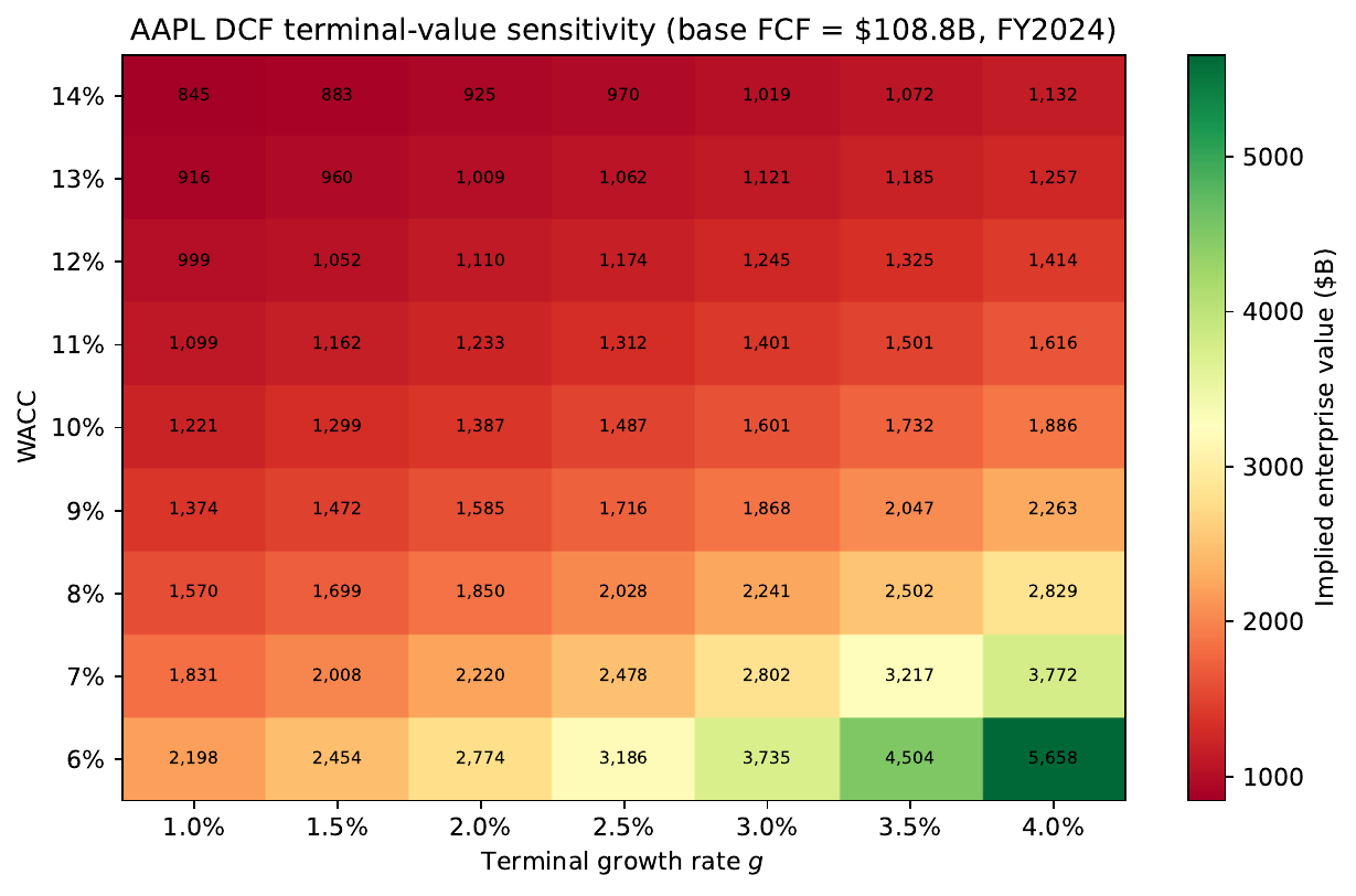
gen_dcf_sensitivity.py; WACC ∈ [6%, 14%], g ∈ [1%, 4%].Comparable selection
The trouble with picking comparables
Multiples are only as good as the peer set. The traditional tools for choosing peers are decades out of date and riddled with well-documented pitfalls.
- Industry codes (SIC, GICS, NAICS) + size filter (0.3–3.0× revenue or market cap): simple, but SIC codes were last revised in 1987. A cloud-computing firm and a 1990s software distributor share a code.
- Diversified conglomerates — a "manufacturing" SIC firm deriving revenue from financial services; its multiples are uninformative for a pure-play manufacturer.
- Cyclical timing — temporarily distressed firms depress the median multiple and undervalue the target.
Embedding-based peers: every candidate is real
Turn each company's MD&A into a dense vector and retrieve the closest ones. Because candidates come from actual filings, no ticker can be hallucinated.
The hybrid pipeline: retrieve, then reason
Neither approach alone is enough. Combine grounded retrieval with qualitative filtering — each used only for what it's good at.
- Candidate generation — the embedding index returns the top 30 by cosine similarity (large enough to capture genuine peers).
- LLM filtering — the model receives candidates + brief descriptions and removes firms that are geographically incomparable, in different competitive positions, or hit by idiosyncratic events (pending acquisition, bankruptcy). Filtered set of 8–12 comparables proceeds to multiple analysis.
End-to-end pipeline: cost, error, and best practices
One input dominates the error in your valuation
Errors flow through a multi-step pipeline. First-order sensitivity analysis shows that one input swamps the rest: the terminal growth rate.
Benchmarking and unit economics at scale
A production pipeline must be evaluated on accuracy and unit economics before deploying across a large coverage universe.
- MAVE (mean absolute valuation error): comparable to the spread between analyst price targets and realised prices — accuracy ceiling is set by unpredictable future cash flows, not the engine
- Coverage rate: above 90% for large-cap companies; above 75% for smaller companies where filings are less standardised
- Directional accuracy: fraction of cases directionally consistent with analyst consensus
- A typical 10-K: ≈50,000 tokens; extraction context 3,000–8,000 tokens per call
- 6 LLM calls per valuation (3 extraction + 1 normalisation + 1 forecast + 1 comparable filter)
- ≈$1–$5 per company at 2024 frontier-model prices (verify current rates at provider pricing pages)
- 3,000 companies refreshed quarterly → ≈$3,000–$15,000 per quarter
- Latency: with parallelised calls, end-to-end ≈ tens of seconds per company
Five best practices for production deployment
- XBRL first — verify extracted numbers against XBRL tags; flag any conflict. LLM extraction is a complement, not a sole source.
- Code interpreter for all arithmetic — no calculation in-context; the generated code is the deliverable and the audit trail.
- Run Monte Carlo — a point-estimate DCF is misleading; communicate the P10–P90 range.
- Mandatory hallucination guards — validate every ticker; trace every figure to its source document (accession number or equivalent); suppress unverifiable claims.
- Human review before publication — the LLM is a powerful assistant, not an autonomous decision-maker. A qualified analyst owns the figures.
What we covered — and where Lecture 6 goes
The LLM-assisted valuation stack
| Component | Key mechanism |
|---|---|
| Data extraction | Filing API (e.g., EDGAR) + LLM table parsing + XBRL validation |
| FCF computation | Code interpreter (deterministic, auditable) |
| Normalisation | LLM reads MD&A; human reviews high-confidence flags |
| Forecasting | CoT prompting; few-shot or LoRA; MAPE / RMSE / DA |
| Scenarios | Bull/base/bear + Monte Carlo over WACC and \(g\) |
| Comparables | Embedding index + LLM qualitative filter (8–12 peers) |
| Orchestration | Multi-agent, parallel specialists, Pydantic contracts |
| Governance | HITL review; hallucination guards; full audit trail |
Lecture 6 — Credit Risk
Key refs: Wei et al. (2022) · López-Lira & Tang (2023) · Hu et al. (2022) · FSB (2023) · IFRS 13 / ASC 820 · IFRS 16 / ASC 842 · Damodaran (2012) · Zhang et al. (2024).
Appendix — case studies, orchestration, and reference tables
A mid-cap SaaS company, valued three ways
A stylised mid-cap US cloud software firm based on a composite of publicly available filings (specific company names and figures are illustrative).
After normalisation (LLM-flagged non-recurring: $45M restructuring + $30M acquired intangible amortisation): EBIT = $915M, FCFF = $789M (τ = 21%).
| Method | Enterprise value | Equity value / share |
|---|---|---|
| DCF (WACC 9%, g 3%) | $17.0B | $57.9 |
| Comparables (9 peers, median EV/EBITDA 24.5×, EBITDA $1.22B) | $29.9B | — |
CoT-generated cash-flow paths for the SaaS case
The CoT forecasting prompt, seeded with historical FCFF and the MD&A summary, returns these base, upside, and bear projections (USD millions).
| Year | Base | Upside | Bear |
|---|---|---|---|
| 1 | 868 | 940 | 760 |
| 2 | 947 | 1,050 | 820 |
| 3 | 1,025 | 1,170 | 870 |
| 4 | 1,100 | 1,280 | 900 |
| 5 | 1,170 | 1,385 | 920 |
How close can a sub-agent pipeline get to the market price?
A complete, agent-orchestrated valuation of Apple Inc. (AAPL) at its FY2024 close (28 September 2024) illustrates how all components connect — and where data-vendor discrepancies emerge.
- FCF from primary 10-K: $108.8B vs. $98.8B from yfinance API — a routine data-vendor gap; primary filings are the authoritative source
- Two-stage DCF → intrinsic ≈ $225/share
- EV/EBITDA cross-check → ≈ $217/share
- 50/50 triangulation → $221.04/share — within 2.6% of the $226.84 market price (inside ±10% tolerance)
Why a multi-agent orchestrator beats one big script
A monolithic pipeline reruns everything when step 6 fails and is untestable in parts. Split it into an orchestrator plus independently testable specialists.
retrieval_agent— filing/source retrieval and extractionfcf_agent— computation and normalisationforecast_agent— CoT projectionscomps_agent— comparable selectiondcf_agent— final valuation and scenario synthesis
FCFF vs. FCFE: which rate discounts which cash flow
The two free-cash-flow definitions are discounted at different rates and yield different value measures. Choose based on capital-structure stability.
| Metric | Discounted at | Yields | When to use |
|---|---|---|---|
| FCFF | WACC | Enterprise value | Stable or changing leverage |
| FCFE | Cost of equity | Equity value directly | Stable leverage only |
Discounting FCFF at WACC gives enterprise value; subtract net debt to recover equity value. Discounting FCFE at the cost of equity yields equity value directly. When capital structure is changing materially, FCFF is more robust because WACC can be held constant while the cost of equity must be re-levered per scenario (Damodaran, 2012).