LLMs for Business Valuation
What this hour looks like
A working session: you audit machine-read financials, design a forecasting prompt, and run a valuation simulation — then we walk the solutions.
- Recap (5 min) — FCFF, the DCF equation, error propagation, evaluation metrics
- Problem 1 (15 min) — audit an LLM's 10-K extraction; propagate the error into the DCF
- Problem 2 (10 min) — design a chain-of-thought forecasting prompt
- Case study (20 min) — run a Monte Carlo DCF; test sensitivity to WACC and \(g\)
- Discussion (5 min) — when is the DCF unreliable, and how do you report uncertainty?
- Solutions (5 min) — walkthrough of Problems 1 and 2
Recap: the machinery you will use
From cash flow to firm value, in two steps
A valuation is just two ideas: figure out the cash the business throws off each year, then add up that cash in today's money.
A tiny growth error is a huge valuation error
The terminal value divides by the gap between the discount rate and the growth rate. When that gap is small, nudging the growth rate even slightly swings the whole valuation.
Make the model narrate before it numbers
A good forecasting prompt forces four stages of reasoning before any number appears — so the logic is visible and checkable.
- Macro — rates, GDP, inflation
- Industry — drivers, headwinds, competition
- Firm — position, CapEx plans, margins from MD&A
- Synthesis — point estimate + P10 downside + P90 upside per year
| Metric | Measures |
|---|---|
| MAPE | Magnitude accuracy |
| RMSE | Sensitivity to outliers |
| DA | Direction for decisions |
Always compare against a random-walk baseline and analyst consensus (Zhang et al., 2024).
Problem 1: audit the machine's extraction
The LLM read a 10-K — but one field is mis-extracted
You pointed an extraction model at a mid-cap industrial's FY2023 10-K. It returned this JSON (USD millions). A classic failure hides inside: it copied CapEx from the cash-flow statement without the parenthesis that marks an outflow, and flattened a footnote.
| Field | Value |
|---|---|
| Revenue | 2,850 |
| EBIT | 428 |
| Depreciation & Amortisation | 195 |
| Capital Expenditure | 240 |
| NWC (FY2023) | 380 |
| Field | Value |
|---|---|
| NWC (FY2022) | 315 |
| Income Tax Expense | 85 |
| EBT (Earnings Before Tax) | 368 |
| Interest Expense | 60 |
| Net New Borrowing | +40 |
Catch the bad field, then price the damage
The extraction figures are on the previous slide. Work through four tasks:
- Audit the extraction. Which textual features of a 10-K make CapEx, parenthesised negatives, or footnoted figures error-prone for an LLM? Name the automated check (e.g. a sign/units cross-check against the cash-flow statement) you would add to catch it.
- Compute FCFF. Using the audited figures, compute FCFF with the effective tax rate (infer it from income tax / EBT). This \(\text{FCFF}_0\) feeds the case study.
- Propagate the error. Recompute the DCF enterprise value (WACC = 10%, 5-yr growth = 6%, terminal growth = 2.5%) with the mis-extracted CapEx vs. the corrected value. How big a valuation error does one bad field cause?
- State a rule. At what extraction-confidence level would you block an automated valuation from reaching a portfolio manager without human review?
Problem 2: design the forecasting prompt
Build a CoT forecasting prompt from MD&A guidance
You are building a valuation agent for the same industrial company. Its MD&A states:
Your tasks:
- Write the four-stage CoT reasoning (macro → industry → firm → synthesis) a well-designed prompt should elicit.
- Identify at least one potential internal inconsistency in the guidance that a consistency-checking step should flag.
- Specify the JSON output format for Year 1–3 FCF forecasts (base, upside, downside, justification).
Case study: the Monte Carlo DCF
What the sensitivity surface looks like
Before drawing thousands of WACC and growth combinations, look at the sensitivity heatmap for a real company — it shows exactly why the distribution shape matters.
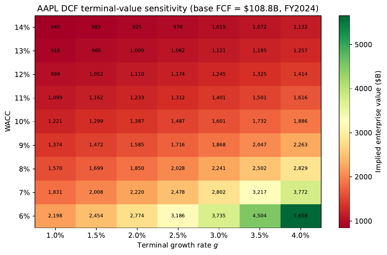
gen_dcf_sensitivity.py; WACC ∈ [6%, 14%], g ∈ [1%, 4%].Replace point estimates with a distribution
Instead of guessing a single WACC and growth rate, you draw thousands of plausible combinations and watch the whole range of enterprise values that results. The base cash flow is your \(\text{FCFF}_0\) from Problem 1.
| Parameter | Mean | Std |
|---|---|---|
| WACC | 10% | 1.5% |
| Explicit growth / yr | 6% | 3% |
| Terminal growth | 2.5% | 1% |
- \(M = 5{,}000\) draws; 5-year explicit horizon;
seed = 42 - Clip terminal growth so \(g_{\text{terminal}} < \text{WACC} - 0.5\%\)
- Report mean, median, std, P10, P25, P75, P90 of the EV distribution
Draw the parameters
First, sample the uncertain inputs and clip terminal growth safely below the discount rate.
import numpy as np

def monte_carlo_dcf(fcff0, g_exp_mean, g_exp_std, wacc_mean, wacc_std,
                    g_term_mean, g_term_std, n=5, M=5000, seed=42):
    rng = np.random.default_rng(seed)
    wacc   = rng.normal(wacc_mean,   wacc_std,   M)
    g_term = rng.normal(g_term_mean, g_term_std, M)
    g_exp  = rng.normal(g_exp_mean,  g_exp_std,  (M, n))

    # Clip terminal growth below WACC -> finite Gordon value
    g_term = np.minimum(g_term, wacc - 0.005)
Each draw is one possible future. The valuation loop follows on the next slide.
Value each draw, collect the distribution
For every draw, grow the cash flows, discount them, add a terminal value, and store the enterprise value.
    ev = np.zeros(M)
    for m in range(M):
        fcfs = [fcff0]
        for t in range(n):
            fcfs.append(fcfs[-1] * (1 + g_exp[m, t]))
        pv_fcf = sum(fcfs[t]/(1+wacc[m])**t for t in range(1, n+1))
        tv = fcfs[n]*(1+g_term[m])/(wacc[m]-g_term[m])
        ev[m] = pv_fcf + tv/(1+wacc[m])**n
    return ev

# Use FCFF0 from Problem 1
ev_sim = monte_carlo_dcf(fcff0=???, ...)
fcff0 with your audited \(\text{FCFF}_0\) from Problem 1 — a wrong extraction here poisons all 5,000 valuations.
Three questions to interrogate your output
- Question A — where does the uncertainty come from? Compare the P10 and P90 enterprise values. What fraction of total EV uncertainty is terminal-value uncertainty vs. explicit-period FCF uncertainty? (Hint: re-run with \(\sigma_g = 0\) to isolate the explicit period.)
- Question B — how sensitive is the headline number? At what terminal growth rate \(g\) does the median EV roughly double relative to the Problem 1 base case? (Hint: solve \(TV \propto 1/(\text{WACC}-g)\) for the target \(g\).)
- Question C — does the market agree? A competitor is acquired at 12× EV/EBITDA. With EBITDA = EBIT + DA = $623M, does the comparables EV fall inside the Monte Carlo P10–P90 range? What does the gap (or its absence) say about pricing?
Fill in this table
| Statistic | Value (USD M) |
|---|---|
| Mean EV | ? |
| Median EV | ? |
| Std Dev | ? |
| P10 (bear) | ? |
| P25 | ? |
| P75 | ? |
| P90 (bull) | ? |
| Derived | Value |
|---|---|
| P90 − P10 range | ? |
| P90 / P10 ratio | ? |
| Comparables EV (12× EBITDA) | ? |
Discussion: communicating uncertainty
When is the DCF unreliable, and how do you report it?
- When \(g \approx \text{WACC}\) — the terminal denominator approaches zero
- When FCF is negative or volatile (e.g. early-stage biotech)
- When the horizon is short, so terminal value dominates
- Point estimate only? Never — why not?
- Point estimate + range (P10–P90)?
- Full distribution histogram?
- Bull/base/bear narrative + Monte Carlo range?
Solutions
One dropped sign, a 3.2× overstatement
- The audit. CapEx, parenthesised negatives, and footnoted figures are the classic LLM extraction traps — the model drops the sign/parenthesis or flattens a note. Fix: a verification sub-agent that cross-checks each figure's sign and units against the cash-flow statement and flags disagreements.
- FCFF (corrected, CapEx as outflow). Effective tax rate \(\tau = 85/368 = 23.1\%\); \(\Delta\text{NWC}=65\), giving \(\text{FCFF}_0 = \mathbf{219.3}\) M.
- Propagated error. If the LLM treats CapEx as \(+240\) (sign dropped), FCFF jumps to 699.3 M — a 3.2× overstatement that flows straight into the DCF (corrected EV ≈ 3,672 M vs. a grossly inflated figure). A single mis-extracted field, not the discounting, breaks the valuation.
- The rule. Block any automated valuation whose extraction confidence is below threshold (or whose sign-check fails) from reaching a portfolio manager without human review.
The firm-stage reasoning — and the tension to flag
- + grid modernisation tailwind supports infrastructure revenue
- − copper/steel bottlenecks compress near-term margins
- + 200-bps margin improvement target over 3 years
- − CapEx at 8–9% of revenue is elevated, limiting FCF conversion
Five things to carry out of this session
- FCFF is not a field in any filing. It is derived from EBIT, DA, CapEx, \(\Delta\)NWC, and the effective tax rate. Each input can carry LLM extraction error, and errors propagate multiplicatively.
- CoT separates narrative from number. Force the model to commit to a macro/industry/firm story before generating numbers — inconsistencies become detectable (Wei et al., 2022).
- Terminal growth dominates the uncertainty. A 100-bps error in \(g\) yields a 15–18% EV error. Report Monte Carlo percentile ranges, not just point estimates.
- Comparables and DCF are complements. A large gap signals either mispricing or a flawed assumption — investigate, don't average.
- Production pipelines need hallucination guards. Validate every ticker; trace every figure to a specific accession number. One hallucinated comparable can distort the whole multiple analysis.
Appendix — stretch problem
Decompose the EV variance, then check the theory
The LLM forecasts the explicit growth path (Problem 2's CoT step), so its forecast error is the uncertainty the model injects. How much of the valuation spread does that error explain?
- Re-run the simulation three times, each freezing two of the three inputs (WACC, explicit growth, terminal growth) at their mean and letting one vary.
- Record \(\mathrm{Var}(EV)\) for each single-input run; express each as a fraction of the all-inputs-varying variance.
- Predict, then check: which input dominates?