Large Language Models in Finance · Chapter 6 / Lecture 6

LLMs for Credit Risk Analysis

Where a smarter model and a defensible model have to be the same model.

Juan F. Imbet · EDHEC Business School / Paris Dauphine – PSL University

Roadmap

Where this lecture is going

The data — what a credit file holds, and the laws that fence it in.
The model — fine-tuning and structured generation to turn a borrower into a default probability.
The household — people don't optimise; LLMs as decision-support, not decision-makers.
Personas — simulating how different borrowers would actually choose.
Governance — evaluation, SHAP, SR 11-7, and shipping a compliant system.

the bigger picture Credit is the one domain where predictive accuracy and regulatory defensibility must be achieved at the same time. Every signal an LLM adds has to survive Fair Lending scrutiny. That tension is the lens for everything that follows.

01

Credit data: sources, privacy, and regulation

The richest behavioural dataset in finance — and one of the most heavily policed.

The founding cautionary tale

Why credit AI is different from everything else

Get a sentiment model wrong and you lose a trade. Get a credit model wrong and you face regulators, lawsuits, and headlines.

the Apple Card incident · 2019 David Heinemeier Hansson's Apple Card limit came in 20× lower than his wife's — despite joint tax returns and comparable profiles. Senator Warren wrote to Goldman Sachs; the NY DFS opened a formal investigation.

Credit data is two things at once

The richest behavioural dataset a bank has
One of the most legally regulated datasets in existence

Both directions carry consequences

Deny unfairly → Fair Lending violations
Extend recklessly → capital losses, systemic risk
Either → regulatory action, litigation, reputational damage

The raw material

What's actually inside a credit file

The three US bureaus — Equifax, Experian, TransUnion — each hold files on roughly 200–230 million adults. A standard file is five kinds of record.

Identification data — name, address history, SSN (encrypted), date of birth
Account data — 24–84 months of payment history per account, plus balance and limit
Inquiry data — hard inquiries (applications) vs. soft inquiries (pre-qualification)
Public records — bankruptcies (7–10 years), civil judgments
Collections — charged-off accounts

The score everyone knows — and its blind spot

FICO records credit behaviour, so it can't see those without any

FICO factor	Weight
Payment history	35%
Amounts owed	30%
Length of credit history	15%
New credit	10%
Credit mix	10%

FICO introduced 1989; VantageScore (joint bureau venture) 2006. Both range 300–850.

the structural limitation Bureau data is circular: it records credit behaviour, so you need credit to build credit. Tens of millions of US adults have thin or no file — recent immigrants, young adults, lower-income households (CFPB, 2013).

Filling the gap — carefully

Alternative data can reach thin-file borrowers, within limits

When the bureau file is empty, lenders look elsewhere — but each new source comes with its own legal leash.

Bank transaction data — cash-flow signals; consent governed by Dodd-Frank §1033
Rent and utility payments — the largest recurring obligation, yet historically invisible to scores
Mobile / telecom data — widely used in emerging markets (airtime top-up, call-graph centrality)
Unstructured text — loan-purpose statements; "medical emergency" ≠ "consolidating payday loans"
Social / behavioural data — largely prohibited; too easily a proxy for protected classes

where the LLM earns its place That unstructured-text row is exactly where a language model adds signal a tabular scorecard can't. The CFPB's Special Purpose Credit Programmes (SPCP) framework allows lenders to proactively use alternative data to extend credit to underserved groups — within ECOA requirements.

The legal fence

Three laws every LLM credit model has to clear

Law	Key constraint for LLM credit models
FCRA (1970)	Adverse action must cite specific reasons (reason codes). A transformer that emits one scalar is not inherently compliant.
ECOA / Reg B (1974)	Prohibits disparate impact on protected classes, not only disparate treatment. Historical data encodes historical bias.
GDPR Art. 22	Right to human review of automated credit decisions (Recital 71). Human-in-the-loop is legally mandated, not optional.

the bigger picture These three rules quietly dictate the architecture: you must explain decisions (FCRA), test for impact (ECOA), and keep a human in the loop (GDPR). Design around them, not after them.

Cleaning before modelling · 1 of 2

Two of the three universal preprocessing traps

Anonymisation

Quasi-identifiers create re-identification risk. Sweeney (2002): 87% of the US population is uniquely identifiable from ZIP + date of birth + sex. Fixes: tokenisation, generalisation (age → bracket), suppression, differential privacy. For LLM text data: NER + entity substitution.

Class imbalance

Default rates run 1–10% over 12 months. With 3% defaults in 1 M rows, "always predict non-default" scores 97% accuracy and is useless. SMOTE (Synthetic Minority Over-sampling Technique) creates new minority-class examples by interpolating between nearby ones; cost-sensitive loss instead re-weights them directly in the objective — the better fit for LLM fine-tuning because SMOTE can't interpolate in token-embedding space.

Give the minority class proportionally more weight so each class has equal aggregate influence on the gradient: \[ w_+ = \frac{n}{2\,n_+}, \qquad w_- = \frac{n}{2\,n_-}. \] Here $n$ is the sample size and $n_+, n_-$ the positive / negative counts. The class ratio no longer decides whose errors the optimiser cares about. In PyTorch: pos_weight argument to BCEWithLogitsLoss.

Cleaning before modelling · 2 of 2

Missing data isn't always missing by accident

The fact that a field is blank can itself be informative — a borrower with no bureau score is telling you something.

MCAR — missing completely at random; simple mean imputation is unbiased
MAR — missing at random (depends on observed data); multiple imputation is consistent
MNAR — missing not at random (depends on the unobserved value itself); needs an explicit model of the missingness

The LLM move

Don't silently impute — serialise the gap into the text so the model can read it: "[INCOME: MISSING] [BUREAU_SCORE: 687]". Gradient-boosted trees (XGBoost, LightGBM) handle MNAR natively via learned optimal branching directions.

02

Credit risk modelling with LLMs

From a 1968 five-ratio score to a language model that reads loan-purpose text.

Fifty years of default models

Where language models fit in a long lineage

Era	Method	Key insight
1968	Altman Z-score	Linear discriminant of 5 financial ratios (66 manufacturing firms)
1974	Merton model	Equity as a call option on firm assets; risk-neutral PD
1990s	Reduced-form	Default as a Poisson intensity process (Duffie & Singleton, 2003)
2015–22	Gradient boosting	Non-linear tabular features; native missing-value handling
Now	Language models	Text-native signals; thin-file borrowers; covenant reasoning

Domain-adapted language models for credit

FinBERT and BloombergGPT showed finance needs its own models

General-purpose LLMs are outperformed on financial NLP tasks by models pre-trained or fine-tuned on domain-specific corpora.

FinBERT (Yang et al., 2020)

BERT fine-tuned on financial news; superior on financial sentiment, NER, and QA tasks. The architecture of choice in published LLM credit-scoring papers: a BERT encoder with a [CLS] head predicts DEFAULT / NO DEFAULT.

BloombergGPT (Wu et al., 2023)

A 50 B-parameter decoder trained from scratch on 363 B financial tokens (Wu et al., 2023). Shows that domain training data compounds benefit beyond general-corpus scale.

three places LLMs add credit value (1) Text-native features — loan purpose, officer notes, news. (2) Thin-file borrowers — heterogeneous alternative data resists tabularisation. (3) Complex commercial credit — covenant reasoning, sector outlook.

Turning a borrower into a prediction

Three ways to fine-tune for default prediction

First write the borrower's profile as a sentence; then pick how the model emits a verdict.

Sequence classification — a BERT encoder with a [CLS] head and sigmoid. The most common choice in published LLM credit-scoring papers (Yang et al., 2020).
Causal LM with label generation — prompt a decoder-only model, read off the label-token probability. Scales to few-shot settings.
Regression on probability — train the model to output a single number, the probability of default. Because a raw 0/1 label is too coarse a training target, you first turn another model's scores into calibrated probabilities (e.g. Platt scaling) and regress against those.

Input serialisation — consistency is critical

Applicant: Age 34. Employment: full-time, 6 years tenure.
Annual income: $58,000. Loan purpose: debt consolidation.
Requested amount: $12,000. Bureau score: 672.
Delinquencies (past 24 months): 1. Assess default risk:

Variation in field ordering or phrasing across training and inference introduces spurious variance.

Training without retraining everything

LoRA: fine-tune a giant model by nudging a tiny slice

A modern language model has billions of internal settings ("weights"). Normal fine-tuning adjusts all of them for your task — slow, storage-heavy, and easy to overshoot when you only have a little data. LoRA leaves the whole model untouched and instead trains a small add-on layer that gently steers its behaviour.

Why it matters for credit

A single lender might have a few tens of thousands of past loans labelled "defaulted" or "repaid" — tiny next to the vast text the base model originally learned from. If you retrain every weight on such a small set, two things go wrong: the model starts memorising your handful of examples instead of learning the pattern (overfitting), and it can forget the general language ability it came with. LoRA sidesteps both: because the original model is frozen and you only train a small add-on, there is far less to overfit and nothing to forget — yet accuracy stays essentially the same as full retraining.

The PD pipeline — from text to decision

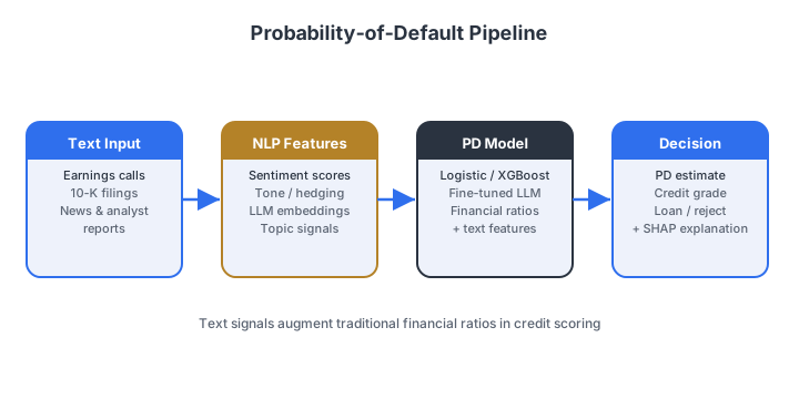
Text in, credit decision out: a four-stage pipeline

Every LLM credit system follows the same logical flow — the complexity hides in each stage, not in the overall architecture.

PD pipeline: text features to PD model to decision — **Figure.** The probability-of-default (PD) pipeline: raw text and structured features are embedded, a fine-tuned LLM produces a raw PD, calibration anchors it to the empirical default rate, and the calibrated PD drives the credit decision together with SHAP reason codes. Source: author illustration.

Making the answer a fixed shape

What is an output grammar?

Left to itself, an LLM can reply with anything — a number, a sentence, a hedge like "probably fairly risky." An output grammar is a set of rules you fix in advance that says exactly what shape the answer is allowed to take. The model still decides what to say, but it can only say it in the form you permit.

Without a grammar

You ask for a default probability and get, unpredictably:

"Around 20–25%, though it depends…"
"HIGH risk."
"0.23"

Your code now has to guess how to read each reply — and sometimes it simply can't.

With a grammar

You declare: the answer must be a single decimal number between 0 and 1, nothing else. Every reply then looks like 0.23 — never a word, never a range, never an apology. The format is guaranteed, so downstream code can always read it.

The intuition

Think of the difference between a blank sheet of paper and a form with labelled boxes. Free text is the blank sheet; a grammar is the form. As the model writes, anything that would break the form is simply not offered as a choice — so a malformed answer becomes impossible, not merely unlikely. That is what lets us reliably turn a "word machine" into a single, well-defined number — the topic of the next slide.

Getting a number out of a word machine

How do you extract a single default probability from an LLM?

The problem

A decoder-only LLM produces a distribution over its entire vocabulary at each position — not a single scalar probability of default. So how do we read off a well-defined PD?

Two routes: (1) constrained decoding — force the model to write a float; (2) verbatim extraction — read logits directly off label tokens.

Using the outlines library:

Define an output grammar — a JSON object with one key "pd" mapped to a float in $[0,1]$.
At each step, intersect the model's next-token distribution with the grammar's automaton.
Renormalise over valid tokens only:

\[ P_{\text{constrained}}(x_{t+1} = v \mid x_{1:t}) = \frac{\exp(\ell_v)\,\mathbf{1}[v \in \mathcal{V}_{\text{valid}}]} {\sum_{u \in \mathcal{V}_{\text{valid}}} \exp(\ell_u)}. \] The model writes {"pd": then produces the float digit by digit. Worked example: if logit for digit "2" is highest at first decimal position, the model generates 0.2..., continuing until the float closes. If it emits 0.23, implied PD = 0.23.

Read that number carefully

The model says "0.10" — but does 10% really default?

We forced the model to output a number that looks like a probability. That doesn't mean the number is true. "0.10" only earns the name "10% chance of default" if, among all the borrowers the model scored 0.10, roughly 10 out of every 100 actually go on to default.

the key point The number is what the model was steered to say, not a measured fact. It reflects the model's internal sense of risk — but there is no guarantee it matches real-world default rates. A model can look confident and still be systematically off (e.g. everyone it scores "10%" actually defaults 25% of the time).

Calibration is the step that checks this and corrects it — making the number mean what it says. That's the next slide.

Making the number mean what it says

Calibration: of everyone scored 10%, do 10% actually default?

A probability is only useful if it matches reality. Plot the model's score against how often that group actually defaulted. On the dashed line, the number is honest.

Each dot is a group of borrowers. The red curve sits above the honest line — the model keeps saying "low risk" when more of them actually default.

Step 1 — check

Points on the dashed line = honest. A point above it (say "10%" that really defaults 25%) means the model is miscalibrated there.

Step 2 — fix

Platt scaling learns a simple stretch-and-shift that bends the red curve back onto the line. Cheap; works with only a few hundred past loans.

how it's built — you do not retrain the LLM The model stays frozen. Platt scaling is a separate one-input logistic regression fit on held-out loans — the whole calibrator is just two saved numbers, re-fit in seconds and versioned apart from the model.

When the bend isn't a straight line

Isotonic regression: more flexible, hungrier for data

Platt assumes the miscalibration is a smooth logistic curve. Isotonic regression makes no such assumption — it just fits any non-decreasing staircase that best matches observed defaults.

Choosing between methods

Platt scaling is preferred for small calibration sets (hundreds of observations) or when the raw score is approximately monotone and log-odds-linear. Isotonic regression is preferred for large sets (thousands) with non-linear miscalibration. Both should be evaluated on ECE and Brier score.

03

Household decisions under uncertainty

Real people don't solve the optimisation — so what should an LLM do for them?

People are not the textbook agent

Why a "rational" borrower is the wrong default assumption

CFPB (2018)

One-third of US mortgage borrowers did not shop before accepting the first offer. Among low-income borrowers the fraction was closer to one-half. The average non-shopper paid about $\$$300/year more in interest — over 30 years, tens of thousands of dollars.

Four reasons households depart from the neoclassical benchmark (Campbell, 2006):

Computational complexity — the full household problem is a high-dimensional stochastic control problem; people approximate
Information asymmetry — knowledge of credit terms, taxes, insurance is required and mostly absent
Dual-process cognition — high-stakes choices often made in fast, affective "System 1" mode (Kahneman, 2011)
Preference inconsistency — hyperbolic discounting, loss aversion, framing effects

A better model of the human

Households satisfice — and that changes the LLM's job

Simon's (1955) bounded rationality Households don't solve the optimisation; they satisfice — searching alternatives until one clears a threshold of acceptability, then stopping. The threshold itself adapts to recent outcomes (aspiration adjustment).

So an LLM that just hands back the "optimal" choice misses the point. The value is in widening the set of alternatives a boundedly-rational household actually considers.

The right division of labour

What a decision-support agent must do — and not do

Three functions, ending with a deliberate restraint.

Information extraction — parse term sheets and insurance exclusions into structured, comparable summaries
Consequence tracing — compute the multi-period financial implications of each choice for this household
Trade-off articulation — present options so the trade-offs are legible without nudging toward one

the autonomy constraint A decision-support agent that consistently recommends the neoclassically optimal choice can undermine household autonomy when stated and revealed preferences diverge. The goal is extension, not replacement, of the household's cognitive frontier.

From principle to plumbing

A practical decision-support architecture

Component	Role
Document ingestion layer	RAG pipeline on term sheets, amortisation schedules, insurance policies → structured JSON
Household profile module	Income, wealth, risk preferences, stated life-stage goals
Consequence engine	Multi-period scenario computations (base, stress, tail)
Dialogue manager	Conversational trade-off presentation; records household's stated rationale

04

Persona agents and behavioural simulation

Conditioning an LLM on a backstory to preview how real borrowers would choose — at origination, and through the life of the loan as their world changes.

Silicon sampling

Give an LLM a backstory, and it answers like that demographic

Argyle et al. (2023)

An LLM conditioned on a detailed demographic backstory reproduces the survey-response distributions of the matching demographic group with striking fidelity. This is an empirical observation about distributional encoding of human-generated text — not a claim about sentience or genuine preferences.

A persona is specified along four axes.

$\Pi = (D, S, \Psi, L)$:

$D$ — demographics: age, sex, household composition, education, region
$S$ — socioeconomics: employment, income, wealth, housing tenure, existing debt
$\Psi$ — psychology: risk aversion $\gamma$, time preference $\delta$, financial anxiety
$L$ — financial literacy: the Lusardi–Mitchell (2011) 3-question battery (interest compounding, inflation, diversification)

A complete specification yields a system prompt of approximately 200–400 words. These four axes are the borrower's stable traits. To simulate behaviour over time, we place the persona in a changing state $s_t$ — income, savings, job, family, home equity — and re-ask the decision each period (see the "life of the loan" slides next).

Two borrowers, two worlds

Meet Maria and Thomas

Maria · 28

Rideshare driver · $\$$2,400/month variable income (range $\$$1,800–$\$$3,200) · $\$$800 savings · one medical collection item · bureau score 584 · no post-secondary education · high security preference.

Thomas · 52

French secondary school teacher · €48,000 salary + spouse €36,000 · €120,000 Livret A savings · 3/3 financial literacy score · moderate risk aversion ($\gamma \approx 2$).

Same loan offer, very different people. Let's watch them choose.

Persona simulation in action

The same loan, reasoned two defensible ways

Scenario: a $\$$20,000 personal loan over 5 years. Option A — fixed 12% APR, $\$$444/month. Option B — variable starting 8% APR, $\$$406/month, capped at 18%.

Maria → Option A (fixed)

"Option B starts lower but says adjustable. Can the payment go up? If it goes to 18%... My rent is $\$$1,200 and some months I barely clear $\$$1,800. I can't risk my payment jumping when work is slow. At least I know exactly what I owe every month."

Thomas → Option B (variable)

"At 8%, five-year interest ≈ €4,300; at 12% ≈ €6,600. If rates stay below ~10% on average, B is cheaper. My wife's income covers fixed obligations. I'd choose B and set aside the monthly difference (€38) into the Livret A as a rate-reset buffer."

the observation Both responses are coherent and defensible. Neither is "wrong." The contrast reflects genuine heterogeneity in risk aversion, income volatility, and financial literacy — all from persona conditioning alone.

The life of the loan, not just the day it's signed

The decision that costs the lender: keep paying — or stop?

Accepting the loan is one choice, on one day. What actually drives losses is the choice the borrower re-makes every month for years: do I keep paying? The same persona setup can simulate that — we let the borrower's circumstances change and simply ask again each period.

Turn the persona into a timeline

Each period, update the persona's state — income, savings, job, family, home equity — then ask: pay in full · pay only part · or miss the payment? Enough consecutive misses is what the lender records as default. Feed the choice back in and roll forward to the next month.

Two very different defaults

Can't pay (liquidity): an income shock and no buffer left. Won't pay (strategic): could pay, but the loan is so far underwater that walking away is rational. Mortgage default often needs both at once — the "double trigger."

why this matters A probability of default is really a claim about the future. Simulating the repayment decision under changing conditions lets us reason about that future borrower-by-borrower — not just fit last year's average onto everyone.

Shock the world, watch them react

Life events and macro shocks you can inject

The real power of the setup: change the borrower's world and watch the decision flip — one persona, many possible futures.

Personal / life events

Job loss or reduced hours
A raise or promotion
A new child · divorce · a move
A large medical or car bill

Macro / market shocks

Rising unemployment (recession)
A rate reset on a variable loan
Inflation eroding real income
A house-price fall → negative equity

the simulation loop draw a shock → update the persona's state → the LLM decides and explains → record it → advance one period. Run the loop across a whole synthetic population and you get a stress-tested portfolio default curve — the same idea as a regulator's recession scenario, but reasoned one household at a time.

A trajectory, not a snapshot

Maria, six months in: a shock hits

Scenario: Maria took the fixed loan ($\$$444/month). In month 6 her rideshare platform cuts driver payouts and a slow winter drops her income to ~$\$$1,500 for two months.

Maria, re-asked at the shock

"$\$$444 is almost a third of what I'm bringing in right now, and rent has to come first — I can't lose the apartment. I'll call and ask if I can pay half for two months; I don't want to just stop and wreck my credit. If they say no… I'd still rather miss this than miss rent."

what the run reveals This is a liquidity risk, not a strategic default — so the right lender response is a short hardship plan, not a collections letter. One simulated trajectory surfaces both the risk and the lever that retains a paying customer.

A worked example

One borrower, month by month, until it resolves

Each month, hand the persona everything at once — income, balances, other bills, life and macro events — and ask: pay in full · pay part · miss? Roll forward until repaid or written off.

The monthly prompt (real state, all at once)

# system (persona + output contract)
You are Maria, 28, a rideshare driver in Ohio,
living month to month — rent and food before debt.
Decide on this month's $444 auto-loan payment.
Reply JSON: {action: PAY_FULL|PAY_PARTIAL|MISS,
amount, reason}
# user (this month — everything at once)
Month 14/60 · take-home $1,510 (usual $2,400)
checking $260 · savings $90
rent $1,200 · other bills $410 · card min $85
events: payout cut 15%; $300 brake repair;
        unemployment 4.3% -> 6.1%
payment due: $444

The model's reply (month 14)

{"action": "PAY_PARTIAL", "amount": 150,
 "reason": "Rent + a $300 repair drained
   my cash; $150 is all I can send."}

…rolled forward month by month

Mo 1 normal → PAY_FULL · Mo 14 shock + repair → PAY_PARTIAL $150 · Mo 16 savings gone → MISS · Mo 18 income recovers → PAY_FULL, catches up → loan survives

and this is where PD comes from Default isn't her choice — it's what the lender records after enough consecutive MISSes. Run thousands of paths (some with harsher shocks) → the fraction ending in default is her probability of default.

05

Evaluation and model risk management

How good is the model — and can you defend it to a validator and a regulator?

Measuring discrimination power

The metrics credit people actually report

Credit modellers don't lead with accuracy — they ask how well scores separate defaulters from non-defaulters. Three measures do that, and they're tightly linked.

AUROC

good > 0.70 · excellent > 0.80 (industry rule-of-thumb)

KS

good > 0.40 · excellent > 0.60

Gini

retail range 0.40–0.70

The supervisory backbone

SR 11-7: an LLM is unambiguously a "model"

SR 11-7 (Fed/OCC, 2011) says every model must be conceptually sound, monitored, independently validated, and documented. LLMs qualify — no exemption. Three pillars, adapted.

Development

Document base-model provenance: corpus, licence, cutoff date
Fine-tune data quality and vintage vs. current cycle
Watch for emergent, untested reasoning

Independent validation

Outcome analysis vs. a logistic baseline
Sensitivity to word order, synonyms, missing fields
Disparate-impact testing by protected class
Adversarial probing

Governance

Versioning: base-model updates may trigger revalidation
Prompt governance: a system-prompt change is a model change
Vendor risk: API models leave residual model risk

Testing for fairness — by the numbers

The Disparate Impact Ratio and the four-fifths rule

ECOA prohibits not just intentional discrimination but also facially-neutral practices with discriminatory effects. The disparate impact ratio (DIR) quantifies this.

The four-fifths rule

Under the regulatory standard, a DIR below 0.80 is treated as presumptive evidence of adverse impact requiring business-necessity justification: \[ \mathrm{DIR} = \frac{P(\text{approve} \mid A = \text{protected})}{P(\text{approve} \mid A = \text{reference})}. \]

why LLMs fail this test A model trained on historically collected data inherits historical discrimination — often in features that appear race-neutral (zip code, loan purpose, occupation category). A complementary measure is the demographic parity difference; both must be evaluated after conditioning on legitimate credit factors, since unconditional gaps may reflect genuine creditworthiness differences.

Explaining a single decision

SHAP turns one prediction into reason codes the law requires

FCRA demands specific reasons for an adverse action. SHAP assigns each feature a fair share of the prediction — borrowed straight from cooperative game theory — and the top contributors become the reason codes. The key property is efficiency: the SHAP values reconstruct the full prediction gap from the baseline.

SHAP, made concrete

Reading a waterfall — and turning it into a notice

A 34-year-old, $\$$58K income, bureau 672, one delinquency. Each feature pushes the predicted default probability up or down from the base rate.

Feature	SHAP $\phi_j$	Running PD
Base value	—	+0.050
Bureau score = 672	+0.041	+0.091
Delinquencies = 1	+0.027	+0.118
Loan purpose: debt consol.	+0.019	+0.137
Income = $\$$58K	−0.012	+0.125
Age = 34	−0.008	+0.117
Employment: full-time 6yr	−0.015	+0.102
Final PD		0.102

compliance, automated The top positive contributors become the FCRA adverse-action reasons — generated directly from the SHAP output. But SHAP values must then be translated into plain language; raw numbers in consumer communications create confusion, not transparency.

06

Deployment and governance

Shipping a credit model that stays auditable, monitored, and humane in production.

The production stack

An architecture built for audit, not just inference

Component	Role
Feature Store	Single source of truth; records retrieval timestamp and source per feature; enables point-in-time reconstruction of any past decision
Inference API	Versioned JSON: raw PD, calibrated PD, reason codes, SHAP values, decision ID, timestamps
LLM Serving	Self-hosted preferred for credit (full data and model control); API-based creates vendor dependency
Decision Record DB	Append-only immutable log; records may be supplemented (outcome) but never overwritten
Monitoring	Data drift (PSI), embedding drift (MMD), score distribution; lagged AUROC by vintage cohort

What the API actually returns

A versioned JSON contract makes decisions auditable years later

Every field in the response is a requirement from some law or supervisory standard — not a developer convenience.

{
  "application_id": "APP-20240315-78423",
  "decision_id":    "DEC-20240315-78423-v2",
  "pd_raw":         0.107,
  "pd_calibrated":  0.102,
  "model_version":  "credit-llm-v2.3.1",          // for revalidation tracking
  "calibration_version": "platt-2024-01",
  "adverse_action_reasons": [
    "Bureau score below threshold",
    "Recent delinquency on record",
    "Loan purpose associated with higher risk"
  ],
  "shap_values": { "bureau_score": 0.041, ... },
  "timestamp_utc":  "2024-03-15T14:23:07Z"
}

Where does the model live?

API-based vs. self-hosted — the credit institution's dilemma

Dimension	API-based	Self-hosted
Latency	200–2,000 ms	50–300 ms
Cost per query	$0.001–$0.05	$0.0001–$0.005
Data control	Partial	Full
Model control	None	Full
Regulatory compliance	Vendor dependency	Institution controls
Infrastructure burden	Low	High

the regulatory preference For credit decisions, self-hosted is preferred because the institution bears full responsibility for the model's outputs regardless of the vendor's data handling practices. An API model's silent update may change outputs without any institution action — a model risk event.

Catching the model going stale

Drift monitoring: is today's population still last year's?

Models decay when the world moves. Two types of drift, two measurement tools.

Tabular features → PSI

Population Stability Index compares input distributions between training and live data. PSI < 0.1: stable; 0.1–0.25: investigate; > 0.25: model review required.

Text inputs → embedding drift

PSI cannot capture semantic shifts in free-text inputs. Maximum mean discrepancy (MMD) or Fréchet distance between sentence embedding distributions is the appropriate measure.

When alerts fire

Three drift severity tiers — from "look" to "stop"

Tiered alerting matches the response to the severity, avoiding both alarm fatigue and silent failures.

Yellow — investigate

PSI > 0.1 on any key input feature
Score distribution mean shift > 0.5 SD

Orange — escalate

PSI > 0.25
AUROC on maturing cohort drops below acceptance threshold
Adverse action rate deviates > 10% from baseline

Red — halt and review

Model output distribution becomes degenerate
API error rate > 1%
Fair lending test fails

Keeping a human in the loop

Three review tiers — and the bias they guard against

GDPR Art. 22, ECOA, and SR 11-7 all require human oversight. Route decisions by difficulty.

Tier 1 · clear approvals

Random quality-control sample only.

Tier 2 · borderline

Active human review before the decision is communicated. PD near threshold, or a high SHAP value on a disputed feature.

Tier 3 · appeals

Full decision record (incl. SHAP waterfall) reviewed; reviewer documents an independent assessment before seeing model output.

automation bias Reviewers anchor hard to a prominently displayed model recommendation. Mitigate: show the recommendation after independent assessment; present SHAP prominently; require documented reasoning before the reviewer sees the model's output.

Paper the regulator needs

The documentation package that ships with the model

MDR — Model Development Report: business need, conceptual framework, data (including base-model provenance and licence), performance, limitations, monitoring plan
MVR — Model Validation Report: independent validation findings, sensitivity analysis, fair-lending analysis, model-risk rating (Low / Moderate / High)
GDPR Art. 22 — plain-language explanation for consumers, translated from SHAP via a constrained LLM; must be comprehensible without financial or technical background
Model Inventory — versioned tracking of base model, fine-tune, calibration, and system prompt

Model change management

What counts as a material model change — and requires revalidation

SR 11-7 requires the model inventory to record every material change. For LLMs the list is longer than for traditional models.

Always a material change

Updating the base model (provider release)
Modifying fine-tuning dataset or procedure
Changing the calibration model
Altering the system prompt or few-shot examples
Changing the structured generation grammar

The silent-update risk

A provider that updates its base model without notice changes the institution's credit decisions without any action by the institution. Versioning contracts, changelog requirements, and automated revalidation triggers are required controls. API-based models create the highest exposure to this risk.

Explaining a denial to a human

SHAP is the input to the explanation, never the output

GDPR Recital 71

The consumer has "the right to obtain human intervention, to express his or her point of view, and to contest the decision." The explanation must be comprehensible to someone with no financial or technical background.

Generated plain-language notice (from SHAP waterfall)

"Your application for a €12,000 personal loan was assessed using an automated system… Factors that increased your estimated risk: your credit bureau score of 672 (below the level typically associated with this product); one late payment in the past twenty-four months; and a loan purpose of debt consolidation. Factors that partially reduced your estimated risk: six years of continuous full-time employment and an annual income of $\$$58,000. You have the right to request human review of this decision…"

Know your failure modes

Five ways an LLM credit model can fail you

Prompt sensitivity — instability under word-order or synonym changes is a red flag; sensitivity analysis is a mandatory SR 11-7 step
Calibration gap — constrained-decoded probabilities reflect internal representation, not empirical default rates; calibration is non-optional
Protected-class proxies — historical text encodes correlations between language, geography, occupation, and protected classes; test for intersectional disparate impact
Adversarial manipulation — a sophisticated borrower may craft text to trigger favourable output; adversarial probing is part of validation
Vendor lock-in and versioning — a silent base-model update changes outputs with no action by the institution; versioning contracts and revalidation triggers are required controls

Wrap-up

The whole stack on one page — and the through-line

Layer	Key design choice
Data	Bureau + alternative; FCRA/ECOA/GDPR; SPCP
Preprocessing	Cost-sensitive loss (not SMOTE); serialised missingness
Modelling	Sequence classification or constrained generation; LoRA
Calibration	Platt (small data) or isotonic; ECE/Brier validation
Household	Persona agents; accept- and repay-decision simulation under life/macro shocks; multi-persona dialogue
Evaluation	AUROC / KS / Gini; DIR / four-fifths rule; SR 11-7
Interpretability	SHAP waterfall → FCRA reason codes → plain language
Serving	Self-hosted preferred; versioned API; append-only record DB
Monitoring	PSI (tabular); MMD (text); three-tier alerting
Oversight	Tier 1/2/3 review; automation-bias mitigations
Documentation	MDR + MVR + GDPR Art. 22 + model inventory

the through-line Credit AI is not merely a prediction problem — it is a regulated sociotechnical system. Every design choice, from the loss function to the API schema, has implications for fairness, explainability, and regulatory compliance.

A

Appendix — extended material

Utility elicitation, population simulation, through-the-cycle validation. Beyond the core lecture.

Appendix A · utility theory

Framing the household choice as expected utility

Underneath "satisficing" sits the classical benchmark: a household picks the action whose expected utility of resulting wealth is highest. Risk aversion is one parameter, $\gamma$.

Appendix A · eliciting preferences

Letting the LLM measure a household's risk aversion

Rather than assume $\gamma$, run a dialogue of lottery choices, find where the household is indifferent, and fit the utility curve to those points.

Present a sequence of binary lottery choices to identify indifference points $(c_j, \lambda_j, g_j)$: certain payoff $c_j$ indifferent to a lottery paying $g_j$ with probability $\lambda_j$ and small floor $\varepsilon$ otherwise.
Extract the stated indifference points from the conversation.
Fit CRRA utility by minimising \[ \hat{\gamma} = \underset{\gamma}{\arg\min} \sum_{j=1}^{J} \big( U_\gamma(c_j) - \lambda_j U_\gamma(g_j) - (1-\lambda_j) U_\gamma(\varepsilon) \big)^2. \]
Use $\hat{\gamma}$ to evaluate the household's alternatives via expected utility.

Quality hinges on the LLM running a coherent multi-turn dialogue without anchoring the responses through framing or order of options.

Appendix B · population simulation

Running many personas to preview a product launch

Draw $N$ personas from a target population and simulate their choices to see which subgroups respond to which product features — before any live test.

Loan uptake modelling — estimate take-up rate vs. APR before an A/B test; compute elasticity $\varepsilon = \Delta\log(\text{take-up})/\Delta\log(\text{APR})$
Mortgage suitability — flag which products create distress risk for Maria-type borrowers while being welfare-enhancing for Thomas-type borrowers
Retirement planning — test auto-enrolment and auto-escalation schemes for low-financial-literacy households (Campbell, 2006: default rules dramatically raise participation)

Appendix B · calibration

A simulation is only useful if it matches a real survey

Validate the synthetic population against the ECB Household Finance and Consumption Survey (ECB HFCS) or the US Survey of Consumer Finances (SCF) before trusting it.

Population alignment — post-stratification weights so the joint attribute distribution matches the target survey
Behavioural alignment — compare simulated vs. survey decision distributions via a calibration loss
Prompt refinement — iterate when calibration loss is high (too generic prompts, wrong product context)

the standard A validated simulation explaining 60–70% of cross-sectional variation is useful. An uncalibrated simulation that claims to predict population behaviour is not.

Appendix C · through-the-cycle validation

Models trained on good times underestimate the bad ones

Concept drift

The feature → default relationship shifts as the economy evolves. A model trained on 2015–2019 data may significantly underestimate default risk in a recessionary environment. Track AUROC and KS across vintage cohorts as outcomes mature.

Population drift

The applicant distribution shifts — new marketing strategy, regulatory change. The model may be accurate on its original population but mis-specified for the new pool.