Portfolio Optimization and Quantitative Trading with LLMs
Where this lecture is going
- Choosing a portfolio — Markowitz's answer, and why naive 1/N beats it: the trouble is estimating \(\boldsymbol{\mu}\) and \(\boldsymbol{\Sigma}\).
- Ways to fix the inputs — shrinkage, factor models, machine learning.
- Black–Litterman — an old, elegant idea: start from the market, tilt by your views, with the math and the intuition.
- Views from an LLM — a worked example: a sentence of text ⟶ a view ⟶ the matrices ⟶ updated weights.
(The rest — LLM trading, backtesting, risk — is in the appendix.)
Classical portfolio theory and its limits
Why does more sophistication lose to a naive 1/N split?
Given many risky assets, how should you split your money? Markowitz (1952) turned this into one elegant optimization. Yet decades later, just putting an equal slice in everything routinely beats the "optimal" answer.
- Sophisticated optimizers chase the efficient frontier
- Naive 1/N equal-weight has no model at all
- 1/N still wins out-of-sample (DeMiguel et al., 2009)
- The theory is right; the inputs are noisy
- Estimating expected returns and covariances dominates the gains
- This is where LLMs enter — sharper inputs from text
Markowitz: trade expected return against risk
Mean-variance optimization picks weights that get the most expected return for a given level of wobble. The famous result: you tilt toward assets with strong return signals and away from risky ones.
Estimation error wins: the inputs are the problem
Plug noisy historical estimates into the optimizer and it confidently makes huge bets on whatever happened to do well lately — then falls apart out of sample.
- Average returns are estimated imprecisely — the noise rivals the signal
- The covariance matrix goes near-singular when assets outnumber history
- Inverting it amplifies those errors into wild weights
- Shrinkage — pull the covariance toward a structured target
- Robust optimization — swap point estimates for uncertainty sets
- Factor models — compress to a few factors (Fama–French 3/5)
Everyone patches the estimates — few change the question being asked
Decades of work attack the noisy \(\boldsymbol{\mu}\) and \(\boldsymbol{\Sigma}\) head-on. These genuinely help — but they still start from history and still hand the optimizer a single point estimate.
- Shrinkage — pull \(\hat{\boldsymbol{\Sigma}}\) toward a structured target (Ledoit–Wolf).
- Factor models — compress to a few drivers (Fama–French), estimating far fewer numbers.
- Robust optimization — optimize against an uncertainty set, not a point.
- Resampling — average optimal weights over bootstrapped inputs.
- Machine learning — forecast returns from many features (trees, nets): powerful, data-hungry, easy to overfit.
- Still just a point estimate fed to the same optimizer.
Black–Litterman: start from the market, not from your guesses
A bit of history. Fischer Black and Robert Litterman built this at Goldman Sachs in the early 1990s precisely because plain Markowitz was unusable on a trading desk — its weights swung wildly on tiny changes to the return estimates. Their fix: don't start from a blank slate. Begin at a neutral, defensible reference — the market — and move away from it only where you hold a genuine, confident opinion, and only as far as that confidence warrants.
- An equilibrium prior — the expected returns already implied by the market portfolio (no history-mining required).
- Your views — specific opinions about returns, each carrying a stated confidence.
Reverse-optimize the market into a set of expected returns
Rather than estimate expected returns from noisy history, ask the reverse question: what expected returns would make today's market-cap portfolio the optimal one? Those implied returns are the starting point — the prior.
If the market weights \(\mathbf{w}^{\text{mkt}}\) are what a representative investor with risk aversion \(\delta\) would hold, then mean–variance optimality, run backwards, pins the returns:
\[ \boldsymbol{\Pi}=\delta\,\boldsymbol{\Sigma}\,\mathbf{w}^{\text{mkt}}. \]We treat \(\boldsymbol{\Pi}\) as the mean of a prior on the true expected returns, with the market's own covariance scaled by a small \(\tau\) measuring how tightly we trust it:
\[ \boldsymbol{\mu}\sim\mathcal{N}\!\left(\boldsymbol{\Pi},\,\tau\boldsymbol{\Sigma}\right). \]- No fragile historical averages — the noisy input that broke Markowitz is gone.
- Automatically diversified and internally consistent with prices.
- A neutral zero-view baseline: believe nothing extra, hold the market.
A view is an opinion about returns — absolute or relative
A view is any statement about expected returns you are willing to back, together with how sure you are of it. Black–Litterman accepts exactly two shapes — and every LLM signal reduces to one of them.
"Asset A will return \(2\%\) next month."
"Asset B will outperform Asset C by \(1\%\)."
Three matrices: the pick matrix \(\mathbf{P}\), the targets \(\mathbf{q}\), the uncertainty \(\boldsymbol{\Omega}\)
Write your \(K\) views as one linear statement about the unknown expected returns \(\boldsymbol{\mu}\), plus noise whose size is your (lack of) confidence:
\[ \mathbf{P}\,\boldsymbol{\mu}=\mathbf{q}+\boldsymbol{\varepsilon}, \qquad \boldsymbol{\varepsilon}\sim\mathcal{N}(\mathbf{0},\,\boldsymbol{\Omega}). \]Worked example — universe \(\{A,B,C\}\), the two views above:
\[ \mathbf{P}=\begin{bmatrix}1&0&0\\[2pt]0&1&-1\end{bmatrix},\quad \mathbf{q}=\begin{bmatrix}2\%\\[2pt]1\%\end{bmatrix},\quad \boldsymbol{\Omega}=\begin{bmatrix}\omega_1&0\\[2pt]0&\omega_2\end{bmatrix}. \]The posterior: a precision-weighted average of the market and your views
Bayes combines the equilibrium prior \(\boldsymbol{\Pi}\) with the views \(\mathbf{q}\) into a single revised vector of expected returns, each side weighted by its precision (inverse variance):
\[ \hat{\boldsymbol{\mu}}_{\text{BL}}= \Bigl[(\tau\boldsymbol{\Sigma})^{-1}+\mathbf{P}^\top\boldsymbol{\Omega}^{-1}\mathbf{P}\Bigr]^{-1} \Bigl[(\tau\boldsymbol{\Sigma})^{-1}\boldsymbol{\Pi}+\mathbf{P}^\top\boldsymbol{\Omega}^{-1}\mathbf{q}\Bigr]. \]- Confident views (small \(\boldsymbol{\Omega}\), large \(\boldsymbol{\Omega}^{-1}\)) pull \(\hat{\boldsymbol{\mu}}\) toward \(\mathbf{q}\).
- Weak views leave it near the market prior \(\boldsymbol{\Pi}\).
- Assets you hold no view on still move, through their covariance with the ones you do.
A sentence from an earnings call becomes an absolute view
"Strong beat likely — raised guidance, accelerating services. Direction: bullish on AAPL. Confidence ≈ 72%."
- Which asset → AAPL
- What return → \(+1\%\) monthly excess (the bullish call, scaled)
- How sure → 72% ⟶ a moderate variance \(\Omega=(0.5\%)^2\)
For a three-name book \(\{\text{AAPL},\text{MSFT},\text{GOOG}\}\), that single absolute view is:
\[ \mathbf{P}=\begin{bmatrix}1&0&0\end{bmatrix},\quad \mathbf{q}=\begin{bmatrix}1\%\end{bmatrix},\quad \boldsymbol{\Omega}=\begin{bmatrix}(0.5\%)^2\end{bmatrix}. \]The equilibrium prior already says \(\Pi_{\text{AAPL}}=0.3\%\).
The view nudges \(\hat{\boldsymbol{\mu}}\), and the optimizer tilts the book
Plugging \(\mathbf{P},\mathbf{q},\boldsymbol{\Omega}\) into the posterior blends the \(0.3\%\) prior with the \(1\%\) view, weighted by confidence:
\[ \Pi_{\text{AAPL}}=0.3\%\ \xrightarrow{\ 72\%\ \text{conf.}\ }\ \hat\mu_{\text{AAPL}}\approx 0.7\%. \]The move — about \(+0.4\) pp — is \(\propto(\mathbf{q}-\mathbf{P}\boldsymbol{\Pi})\) and shrinks back toward the prior as \(\Omega\) grows. MSFT and GOOG, with no view of their own, still shift a little through their covariance with AAPL.
In the literature: Mantshimuli & Mwamba (2025) fold multi-LLM sentiment views into Black–Litterman and improve Sharpe over single-LLM and market-cap benchmarks.
| Weight | Before (market) | After (BL) |
|---|---|---|
| AAPL | 6.0% | 9.1% |
| MSFT | 5.0% | 4.4% |
| GOOG | 4.0% | 3.6% |
Illustrative weights on a three-name book. One confident view tilts toward AAPL and funds it from the rest — a measured tilt, not a corner bet.
A second kind of view: one name will beat another
Comparison is what an LLM does best. Rather than pin an absolute level, it can judge that one name will out-earn a peer — a relative view.
"AAPL will outperform MSFT by \(\approx 0.8\%\) next month" becomes a row that is \(+1\) on the winner and \(-1\) on the loser:
\[ \mathbf{P}=\begin{bmatrix}1&-1&0\end{bmatrix},\quad \mathbf{q}=\begin{bmatrix}0.8\%\end{bmatrix},\quad \boldsymbol{\Omega}=\begin{bmatrix}(0.4\%)^2\end{bmatrix}. \]- Two peers, side by side — read both earnings calls and compare guidance tone and demand commentary.
- Share-shift narratives — one firm taking share from another (product cycle, pricing, launches).
- Supply-chain links — a supplier's raised guidance implying a customer's cost or a rival's squeeze.
- Cross-section of a sector — who is raising vs. cutting guidance across an industry's filings.
- Relative sentiment — analyst-note and news tone for A minus B, not A alone.
Don't ask the LLM for a precise return — ask it for a distribution
The weakest link above is the number itself. An LLM that types "\(+1.0\%\)" is inventing a point estimate: it is not a calibrated regressor, the figure is prompt-sensitive and anchored, and it hides its own uncertainty. Both \(\mathbf{q}\) and \(\boldsymbol{\Omega}\) deserve better.
Then \(\mathbf{q}\) and \(\boldsymbol{\Omega}\) fall out of the distribution itself:
\[ q=\sum_k p_k\,r_k, \qquad \Omega=\sum_k p_k\,(r_k-q)^2. \]A peaked distribution ⟶ small \(\Omega\) ⟶ a confident view; a flat one ⟶ large \(\Omega\) ⟶ the posterior barely moves. Confidence is now measured, not asserted.
Lecture 10 — four takeaways
- The optimizer was never the weak link. Estimating \(\boldsymbol{\mu}\) and \(\boldsymbol{\Sigma}\) is — which is why naive 1/N, estimating nothing, so often wins.
- The standard fixes patch the estimates. Shrinkage, factor models, and machine learning all help, but still hand the same optimizer point estimates drawn from history.
- Black–Litterman reframes the problem. Start from the market's implied returns and tilt by views weighted by confidence; with no views you simply hold the market.
- A view is just \((\mathbf{P},\mathbf{q},\boldsymbol{\Omega})\). An LLM can produce one from a sentence of text — and the map confidence ⟶ \(\boldsymbol{\Omega}\) is what stops a noisy signal from running the book.
Appendix — extended derivations, benchmarks & further reading
Where LLMs can — and cannot — add value
Be honest about the edge. LLMs shine at turning messy text into structured signals; they are not magic return predictors or covariance estimators.
- Structuring alternative data (calls, filings) into factors/views at scale
- Risk monitoring — flagging emerging risks before the statements show them
- Analyst-view aggregation with calibrated uncertainty
- Return prediction beyond a few days (factor risk dominates)
- Replacing factor models (not built to estimate covariances)
- Timing in isolation (no order-flow / microstructure access)
LLMs as alternative-data processors
Text is the least-saturated alternative data
Satellite imagery and credit-card flows lose their edge fast once everyone buys them. Text — earnings calls, reports, filings, news, central-bank speak — pours out terabytes a year and stays comparatively un-mined.
- Views for Black–Litterman — a per-firm view with calibrated uncertainty.
- Factors for Fama–French — a long-short "language factor" tested for alpha.
A four-stage pipeline for extracting analyst views
Each document becomes a single number — a view — through a disciplined assembly line that ends with a sanity-preserving normalization step.
- Retrieve & chunk — pull from a feed or SEC EDGAR, split semantically
- Score — an LLM (or FinBERT) assigns sentiment per chunk
- Aggregate — position-weighted into a document signal in \([-1,1]\)
- Normalize — within industry and period to remove sector trends
Analyst-report tone carries incremental return information (Lehavy, Li & Merkley, 2011); this pipeline operationalises that insight at scale with an LLM.
Earnings-call views across 100 S&P 500 names
Give the model an analyst's job description and one rule: read the excerpt, output a single number from bearish to bullish.
"You are a sell-side equity analyst. Given this earnings-call excerpt, assign a return sentiment score from −1 (bearish) to +1 (bullish) over the next month. Output only the number."
- CFO "raising full-year guidance 5%, no demand softening" → score ∈ [0.6, 0.9]
- CEO "cautious on macro, right-sizing cost structure" → score ∈ [−0.6, −0.3]
Calibrated on \(T=800\); BL optimizer with \(\delta=3,\ \tau=0.05\).
Meskovskis & Kenyon (2024): an LLM-generated SWOT view from strategic filings supports longer horizons where price-based backtesting lacks power.
Building a "language factor" — and asking if it earns alpha
Rank every stock by its text signal, go long the most bullish and short the most bearish, and you have a tradeable factor. The real test: does it pay beyond the well-known factors?
The factor zoo — and why automated search makes it worse
Test hundreds of candidate factors on one history and some will look profitable by pure luck. Letting an LLM generate even more candidates multiplies that danger.
- AlphaQuant (Yuksel, 2025): an LLM-evolutionary loop that proposes, evaluates, and refines alpha features — replacing manual feature engineering.
- This amplifies the multiple-testing problem: the backtesting discipline that follows becomes non-negotiable.
LLM-guided algorithmic trading
Where in the trading stack do LLMs belong?
Trading runs from microsecond high-frequency to multi-week macro. LLMs matter in the slow regime — where signal quality, not delivery speed, decides performance. Think latency in hours, not milliseconds.
- scale with signal strength,
- stay bounded (no runaway concentration),
- decay as the signal ages.
From a raw sentiment score to a dollar-neutral position
Standardize the model's output against its own recent history, then size positions so the book is long the bullish names and short the bearish ones in equal measure — insulated from the overall market.
Kirtac & Germano (2024): GPT-3-class news scores predict next-day returns with above-chance directional accuracy and a high in-sample post-cost Sharpe — but single-sample Sharpes rarely replicate out of sample. A magnitude baseline, not a promise.
LLMs as an extra sense for order execution
When you must buy or sell a large block, the question is how fast. Classical theory balances market impact against the risk of waiting; an LLM adds a warning light, not a new steering wheel.
HARLF (Coriat & Benhamou, 2025): three-tier hierarchical RL injecting LLM sentiment into the reward — strong risk-adjusted returns on 2018–2024 data.
Why LLMs are not stock pickers
A statistically significant signal is not the same as a profitable one. Markets — especially for big, heavily-watched stocks — are simply too fast and too crowded.
- Semi-strong EMH (Fama, 1970): public info is already in prices; large caps adjust to news in minutes — faster than an LLM API can read it.
- Grossman–Stiglitz: some return must accrue to informed trading, but if everyone subscribes to the same API the signal crowds and alpha compresses.
- Calibration problem: a "70% positive" LLM probability is not a claim the stock rises 70% of the time — it requires out-of-sample calibration to returns.
Backtesting with LLM signals
A backtest is necessary, never sufficient
A backtest asks: would this have made money historically? A realistic one also accounts for trading frictions, data limits, and the fact that you tried many strategies. An in-sample Sharpe is nearly useless — the model has already seen the future.
- Train on a block of past data
- Validate on the next window — hyperparameters only
- Test on the next step; report performance only on concatenated test windows
Out-of-sample Sharpe — and the costs that eat it
Judge a strategy on risk-adjusted return earned on data it never saw. Then subtract the bill: trading frequently can quietly erase the very edge you found.
- Rule of thumb: Sharpe > 1.5 over ≥ 3 years OOS before paper trading
- Cost components: bid–ask (single-digit bps large-cap, tens small-cap), market impact, financing (> 5% p.a. on hard-to-borrow)
- Capacity: trade ≤ 5–10% of average daily volume; earnings-call signals crowd in the first hours
Look-ahead and survivorship: how good backtests go wrong
Two biases quietly inflate nearly every naive backtest — and LLMs introduce subtle new ways to leak the future into the past.
- Embedding leakage — model fine-tuned on transcripts post-dating the trade
- Model-selection leakage — best variant chosen by full-period performance
- Timestamp errors — calls release after close; day-\(t\) open uses unavailable info
Risk management applications
Textual warnings shift risk before they hit prices
Management caution, litigation, sovereign stress — these qualitative warnings fatten the bad tail of the return distribution before they show up in the numbers. LLMs read this stream and feed it into volatility and tail-loss estimates in near real time.
Automatic de-risking when the text turns dark
Wire the risk signal directly into the optimizer: as the language around a sector turns negative, its modeled risk rises, the risk constraint tightens, and the system trims exposure on its own.
- Ingestion — poll EDGAR, news APIs, social at a configurable frequency
- Classification — LLM emits structured JSON
(
risk_level,risk_type,affected_positions) - Action — route critical alerts to a risk officer or a pre-approved auto-response
Calibration: tune to the firm's portfolio; beat alert fatigue (< 20/day for 100 positions); match latency to use (minutes EOD, seconds intraday).
An 8-K alert that cut half the loss
4:17 PM — a held name files an 8-K announcing an SEC investigation into revenue recognition. Within 30 seconds the LLM classifies it.
{ "risk_level": "critical", "risk_type": "legal",
  "affected_positions": ["TICKER_X"],
  "summary": "SEC formal order into revenue recognition.
              Historical precedent: 20-40% downside risk." }
The action layer cuts the position from 2.1% → 1.0% at the next open. Next morning the stock opens −28%.
The Sharpe-ratio geometry of the frontier
The tangency portfolio is the single point that maximizes return per unit of risk — and a deterministic plot shows it sitting almost on top of the naive 1/N portfolio.
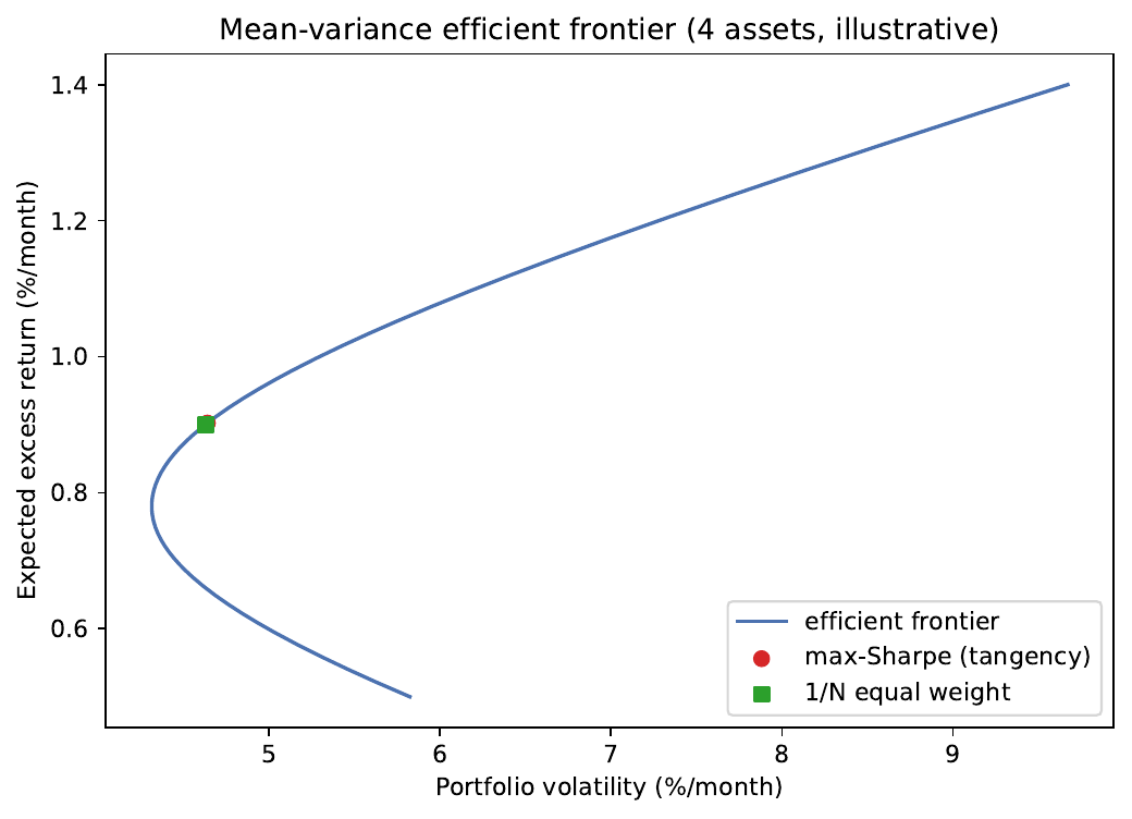
gen_efficient_frontier.py (no data or network dependence).- Adding the non-negativity constraint removes the closed form; the mean-variance program must then be solved numerically as a quadratic program.
A map of recent LLM-portfolio research
| Work | Mechanism | Result |
|---|---|---|
| Mantshimuli & Mwamba (2025) | Multi-LLM → LSTM → BL views | Sharpe / return ↑ vs. single-LLM |
| Yuksel (2025), alpha | LLM evolutionary tournament | Portfolio selection, large universes |
| Yuksel (2025), AlphaQuant | LLM-evolutionary factor search | Automated alpha-feature discovery |
| Coriat & Benhamou (2025) | HARLF: 3-tier hierarchical RL | Strong risk-adj. returns 2018–2024 |
| Meskovskis & Kenyon (2024) | SWOT views from strategic filings | Long-horizon view generation |
| Saha, Lyu et al. (2025) | Survey of agentic PM systems | Taxonomy + open benchmarks |
Practitioner survey: Mann (2024) — durable value sits in the information-extraction layer, not the decision layer.
News, volatility, and what the EMH literature shows
- Tetlock (2007): dictionary sentiment from a newspaper column predicted excess returns over a decade ago — so the incremental value of LLMs over dictionaries is the relevant comparison; broad-coverage signals have decayed.
- NVIX (Manela & Moreira, 2017): a text-based disaster-risk measure from newspaper archives predicted market variance and crash risk. LLMs push this to firm-level, real-time.
- Regulatory context: Fed SR 11-7 requires model outputs be explainable, validated, and auditable — directly binding on LLM risk signals (see the RegTech chapter).
Why view uncertainty shrinks as the signal grows
The rule that ties confidence to signal strength is what keeps a loud-but-weak model from hijacking the portfolio — and it must be calibrated only on past data.